Bioimpacts. 2025;15:30849.
doi: 10.34172/bi.30849
Original Article
A hybrid transformer-based approach for early detection of Alzheimer’s disease using MRI images
Qi Wu Data curation, Formal analysis, Investigation, Methodology, Writing – original draft, Writing – review & editing, 1 
Yannan Wang Conceptualization, Data curation, Formal analysis, Investigation, Methodology, Project administration, Supervision, Validation, Visualization, Writing – review & editing, 2, *
Xiaojuan Zhang Formal analysis, Investigation, Supervision, Validation, Visualization, Writing – review & editing, 1
Hongqiang Zhang Formal analysis, Investigation, Project administration, Validation, Visualization, Writing – original draft, Writing – review & editing, 3
Kuanyu Che Data curation, Validation, Writing – original draft, Writing – review & editing, 4
Author information:
1Department of Psychiatry, The Third People's Hospital of Lanzhou, Lanzhou 730030, Gansu, China
2Department of Pediatric Psychiatry, The Third People's Hospital of Lanzhou, Lanzhou 730030, Gansu, China
3Department of Traditional Chinese Medicine, The Third People's Hospital of Lanzhou, Lanzhou 730030, Gansu, China
4Department of Magnetic Resonance Imaging, The First People's Hospital of Lanzhou, Lanzhou 730030, Gansu, China
Abstract
Introduction:
Alzheimer's disease (AD) is a progressive neurodegenerative disorder that poses significant challenges for early detection. Advanced diagnostic methods leveraging machine learning techniques, particularly deep learning, have shown great promise in enhancing early AD diagnosis. This paper proposes a multimodal approach combining transfer learning, Transformer networks, and recurrent neural networks (RNNs) for diagnosing AD, utilizing MRI images from multiple perspectives to capture comprehensive features.
Methods:
Our methodology integrates MRI images from three distinct perspectives: sagittal, coronal, and axial views, ensuring the capture of rich local and global features. Initially, ResNet50 is employed for local feature extraction using transfer learning, which improves feature quality while reducing model complexity. The extracted features are then processed by a Transformer encoder, which incorporates positional embeddings to maintain spatial relationships. Finally, 2D convolutional layers combined with LSTM networks are used for classification, enabling the model to capture sequential dependencies in the data.
Results:
The proposed framework was rigorously tested on the Alzheimer's Disease Neuroimaging Initiative (ADNI) dataset. Our approach achieved an impressive accuracy of 96.92% on test data and 98.12% on validation data, significantly outperforming existing methods in the field. The integration of Transformer and LSTM models led to enhanced feature representation and improved diagnostic performance.
Conclusion:
This study demonstrates the effectiveness of combining transfer learning, Transformer networks, and LSTMs for AD diagnosis. The proposed framework provides a comprehensive analysis that improves classification accuracy, offering a valuable tool for early detection and intervention in clinical practice. These findings highlight the potential for advancing neuroimaging analysis and supporting future research in AD diagnostics.
Keywords: Alzheimer’s disease, Multimodal, Transfer learning, Transformer networks, Recurrent network, MRI images, Feature fusion
Copyright and License Information
© 2025 The Author(s).
This work is published by BioImpacts as an open access article distributed under the terms of the Creative Commons Attribution Non-Commercial License (
http://creativecommons.org/licenses/by-nc/4.0/). Non-commercial uses of the work are permitted, provided the original work is properly cited.
Funding Statement
This work was supported by Application of MRI-based hippocampal structural and functional changes in the diagnosis of Alzheimer's disease: A research study(Gansu Provincial Natural Science Foundation 22JR5RA1066).
Introduction
Alzheimer's disease (AD) is one of the most significant and complex neurodegenerative disorders, gradually leading to the loss of cognitive abilities and memory in affected individuals. Predominantly affecting older adults, it is recognized as the most common form of dementia. With the increase in life expectancy and the aging global population, the prevalence of Alzheimer's is expected to rise significantly in the coming decades. This underscores the critical need for early detection and diagnosis, as timely therapeutic interventions and disease management can improve patients' quality of life and reduce the societal and economic burden of the disease.1,2
Traditional methods for diagnosing Alzheimer's rely on clinical tests, cognitive assessments, and medical imaging techniques such as MRI and PET scans.3 While these approaches can be effective in some cases, they are often dependent on detecting the disease at its later stages and are less capable of identifying it in its early phases. This has highlighted the need for innovative and intelligent approaches to achieve more accurate and timely diagnosis. In this regard, artificial intelligence (AI), particularly machine learning (ML) and deep learning algorithms, has emerged as a powerful tool capable of analyzing vast amounts of data to identify subtle patterns that are difficult for humans to detect.4,5
Despite the potential of AI in diagnosing Alzheimer's, several challenges remain. One of the most critical issues is the limitation and quality of available data. Data used to train AI models must be accurate, diverse, and representative of the disease's many facets to ensure good performance in real-world conditions. The scarcity of such data, especially longitudinal data that tracks the disease's progression over time, poses a significant barrier. Additionally, individual differences in brain structure and the rate of disease progression require AI diagnostic models to be more personalized to account for these variations.6
Another significant challenge is the interpretability of the results. Many deep learning models operate like "black boxes," making it difficult to explain the reasoning behind their decisions. This lack of transparency can hinder the adoption of AI technologies by medical professionals, as in the medical field, the ability to explain and trust the decision-making process is crucial.7,8
Furthermore, integrating AI technologies into existing medical systems and utilizing them in clinical settings poses another challenge. AI methods not only need to be highly accurate but must also seamlessly fit into the workflow of healthcare professionals, serving as an assistive tool in clinical decision-making processes.
In conclusion, while significant progress has been made in utilizing AI for Alzheimer's diagnosis, further research and development are needed to overcome existing challenges. Improving data quality, enhancing the interpretability of AI models, and better integration with healthcare systems are essential steps toward realizing the full potential of AI in this field.9,10
Alatrany et al11 present a machine learning model that classifies AD with high accuracy while also providing interpretable explanations for its decisions. This approach addresses the common "black box" problem in AI models, enhancing their trustworthiness in clinical settings
Researchers presented a machine learning framework that significantly enhances the predictive capability of brain MRI data. They employed the unsupervised learning algorithm of local linear embedding (LLE) to reduce multivariate MRI data regarding regional brain volume and cortical thickness into a lower-dimensional space, while retaining the global nonlinear structure. The extracted brain features were then utilized to train a classifier for predicting future conversion to AD based on baseline MRI scans.12
In Altaf et al study,13 multi-class AD classification is achieved by integrating both image and clinical features. Researchers developed a framework that combines advanced machine learning algorithms to analyze MRI images alongside clinical data, improving diagnostic accuracy. The approach aims to effectively distinguish between various stages of AD, ultimately enhancing patient management and treatment strategies. Alam and colleagues utilized the ADNI dataset for AD diagnosis. They extracted various features from images using LDA and KPCA and performed classification with a multi-kernel SVM. This approach enhances diagnostic accuracy and helps differentiate between various stages of AD.14
Researchers employed a multi-diagnostic approach using machine learning for the early diagnosis of AD, focusing on generalizability across diverse patient populations. They developed a framework that integrates data from multiple sources, significantly enhancing the model's effectiveness in identifying early signs of the disease. This strategy effectively addresses the limitations of traditional diagnostic methods and provides a reliable, scalable solution, ultimately improving the potential for early intervention in various clinical settings.15
Tripathi et al,16 developed a method for classifying six types of cognitive impairment, including AD, using speech-based analysis. By analyzing speech data from DementiaBank’s Pitt Corpus with five machine learning algorithms, the study achieved a 75.59% overall accuracy, with XGBoost performing better than other algorithms, except for random forest. This innovative approach highlights the potential for creating a non-invasive and cost-effective diagnostic tool for the early detection and management of cognitive impairments, enhancing clinical practices in this critical area of healthcare.
Deep learning techniques have been increasingly used for diagnosing and classifying AD due to their ability to analyze complex medical imaging data, such as MRI and PET scans. Convolutional neural networks (CNNs) are particularly effective in extracting features from brain scans, helping to detect early signs of the disease. These models are capable of achieving high accuracy in classification tasks, often outperforming traditional methods. However, challenges remain in interpretability, the need for large datasets, and ensuring generalization across different populations.17,18
In recent advancements, automated AD classification has seen improvements through the integration of deep learning models, particularly with the use of Soft-NMS (Soft Non-Maximum Suppression) and an enhanced ResNet50 architecture. This approach refines traditional classification methods by optimizing feature extraction and reducing false positives during the classification process. Soft-NMS enhances the model's ability to differentiate between subtle disease markers, while the improved ResNet50 boosts accuracy and efficiency in detecting Alzheimer's from medical imaging data, making the diagnosis process more reliable.19 Researchers employed a densely connected CNN with a connection-wise attention mechanism to learn multi-level features from brain MRI images for AD classification. The method extracts multi-scale features from pre-processed images, transforming them hierarchically into compact high-level features by combining connections from different layers. Additionally, the convolution operation is extended to 3D to capture spatial information. The approach is evaluated on MRI data from 968 subjects in the ADNI database for effective classification.20
The use of deep neural networks based on convolutional networks has garnered significant attention from many researchers.21-25
In Ebrahimi and Luo study,21 a CNN, consisting of 2D convolutional and pooling layers, was utilized for AD detection. The dataset was divided for testing and training, with 70% allocated for training and 30% for testing. Results indicate that the proposed method demonstrates good performance. Samhan et al22 have proposed a machine learning method for the early diagnosis of AD and mild cognitive impairment (MCI) using high-resolution MRI. They analyzed regional morphological differences in the brain, achieving 96.5% accuracy in distinguishing mild AD from healthy subjects, 91.74% for differentiating progressive MCI, and 88.99% for classifying progressive MCI versus stable MCI. The approach focuses on macroscopic shape differences between groups, enhancing discrimination power.
Mehmood et al26 developed a Siamese convolutional neural network (SCNN) model inspired by VGG-16 to classify dementia stages in AD. They addressed issues of overfitting due to limited image samples by using data augmentation techniques. Testing on the OASIS dataset, their approach achieved an impressive accuracy of 99.05%. The proposed model outperformed state-of-the-art models in terms of performance, efficiency, and accuracy, demonstrating the effectiveness of machine learning in early AD diagnosis and dementia classification.
Given that deep CNNs (DCNNs) have many parameters and training these networks with a limited amount of data can be challenging, researchers have utilized transfer learning techniques. These methods allow for leveraging pre-trained models on larger datasets, which can enhance performance and reduce the need for extensive training data in specific applications, such as AD classification.27
In the research presented in Acharya et al,28 the focus is on classifying MRI scans of AD patients into multiple categories by utilizing VGG16, ResNet-50, and AlexNet as transfer learning models, alongside CNNs. The goal is to enhance classification accuracy and effectively differentiate between various stages or types of AD based on MRI data.
However, using these methods alone is not sufficient. Therefore, researchers29-32 have employed ensemble learning techniques to improve the detection rate. By combining the strengths of multiple models, ensemble methods enhance classification accuracy and provide more robust predictions for AD diagnosis. In Khanna study,31 the method proposed for multi-level classification of AD utilizes DCNNs in conjunction with ensemble deep learning techniques. This approach combines the outputs of multiple models to enhance classification accuracy and improve detection rates, allowing for more robust differentiation among various stages of the disease.
Recently, transformer-based methods have garnered attention due to their ability to capture complex dependencies in data, outperforming traditional CNNs and transfer learning approaches, particularly in handling multimodal data and missing information.33-35
Liu et al36 presented cascaded multi-modal mixing transformers for AD classification, effectively integrating various data modalities to enhance accuracy. The model demonstrates robustness against incomplete data, achieving improved performance in distinguishing different stages of AD, showcasing its potential utility in clinical applications. Li et al,37 introduced Trans-ResNet, an innovative architecture that merges the advantages of CNNs and transformers to enhance brain disease classification from MRI data. This model addresses CNNs' limitations in capturing global dependencies and was pre-trained on a large brain age estimation dataset. A model integrating CNN with shift window attention for enhanced classification of AD has been proposed. This method harnesses the strengths of both architectures, improving feature extraction and understanding of global context. The model showed promising results in accurately distinguishing between various stages of AD, highlighting its potential to advance diagnostic accuracy in clinical settings.38
In AD diagnosis, traditional methods often rely on handcrafted features and classical machine learning models such as support vector machines (SVMs) and decision trees. These methods are typically limited in their ability to capture complex, non-linear features and model intricate temporal and spatial relationships in imaging data. Moreover, many of these approaches depend on a single view of the data (usually a subjective perspective), which restricts the model's ability to extract rich, multi-dimensional information.
In contrast, our proposed approach leverages an advanced combination of transfer learning, transformer networks, and LSTM to effectively extract complex features and model both temporal and spatial dependencies. The use of ResNet50 for local feature extraction, along with Transformer networks to preserve spatial relationships and LSTM networks for capturing temporal dependencies, significantly enhances the system's diagnostic accuracy. Furthermore, the use of three distinct MRI views (sagittal, coronal, and axial) provides a richer representation of brain structure, leading to improved diagnostic performance.
Considering the challenges in early AD diagnosis and the limitations of current methods, we propose a hybrid approach utilizing transformer networks for analyzing MRI images. This method involves the collection of MRI images from multiple angles to enhance data diversity. Features are extracted using transformer networks for each angle and then combined in the classification stage. Finally, recurrent and fully connected layers are employed for classification. This approach allows for a better understanding of the disease and aims to improve diagnostic accuracy. Our proposed approach introduces several innovations for early AD diagnosis. First, it employs a multi-modal strategy that utilizes MRI images from various angles to enhance data diversity. Second, we utilize an improved transformer-based network, which allows for more effective feature extraction and context understanding. Finally, the method incorporates an end-to-end framework, facilitating a seamless transition from feature extraction to classification. This comprehensive approach aims to significantly improve diagnostic accuracy and provide a deeper understanding of the disease. The main contributions of this paper are summarized as follows:
Overcomes limitations of handcrafted feature extraction: Traditional methods rely on manual feature selection, which is often insufficient for capturing complex, non-linear patterns in Alzheimer's imaging data. Our method utilizes deep learning-based feature extraction through ResNet50, enhancing the quality of extracted features.
-
Addresses limited ability to model temporal and spatial relationships: Existing methods struggle to model both spatial and temporal dependencies in MRI data. Our approach combines Transformer networks (for spatial relationships) and LSTM networks (for temporal dependencies), enabling a more comprehensive understanding of Alzheimer's-related brain changes over time.
-
Improves diagnostic accuracy by using multimodal MRI views: Traditional methods typically rely on a single MRI view, limiting the information captured. We use sagittal, coronal, and axial views, providing a richer and more detailed representation of brain structures, which enhances the model's diagnostic performance.
-
Reduces model complexity with transfer learning: By using pre-trained networks like ResNet50, we minimize the need for large datasets while maintaining high accuracy, addressing the issue of overfitting and reducing training time compared to traditional deep learning models.
-
Achieves superior performance compared to existing methods: Our method demonstrates a significant improvement in diagnostic accuracy (96.92% on test data, 98.12% on validation data) compared to traditional and other state-of-the-art methods in Alzheimer's detection, providing a more reliable tool for early diagnosis.
Methods
Given that feature extraction from MRI images is essential for the diagnosis of AD, this paper employs a multi-faceted approach for feature extraction. In the proposed method, images are utilized from three different perspectives: lateral, superior, and posterior views of the head. We applied several techniques to ensure optimal input data for the model. First, all MRI images were resized to a consistent size to ensure uniformity across the dataset. We performed normalization by scaling pixel values to the range [0, 1] to standardize the intensity values and reduce model bias due to varying image scales.
To extract features from these images, transfer learning is implemented, significantly reducing the number of model parameters. This decrease in parameters lowers the risk of model overfitting and enhances the quality of features extracted from the images. The model used in this phase is based on ResNet architectures.
Next, the output from the last layer of the ResNet network, which consists of images sized 16 by 16 pixels, is utilized. These images are constructed based on the various perspectives. They are treated as batches that need to be aggregated with positional embeddings before entering the subsequent module. This next module focuses on extracting local features using transformer encoder layers. These layers employ an attention mechanism to extract relevant features from the images. After the transformer module, the resulting feature vector-comprising rich, high-level features-is resized and combined with the features from various layers of the ResNet network. This process ensures that both detailed and low-level features are retained. Following this, a classification module is implemented. In this module, suitable features are initially extracted from the various images generated using the CONV2D layers. Since there exists a sequential relationship between the data and the generated images, LSTM layers are utilized to extract the most relevant features. Finally, in the concluding module, two pooling layers are applied to reduce parameter dimensions, followed by a fully connected layer for classification. Fig. 1 illustrates the overall stages of the proposed method, which we will detail further in the following sections.
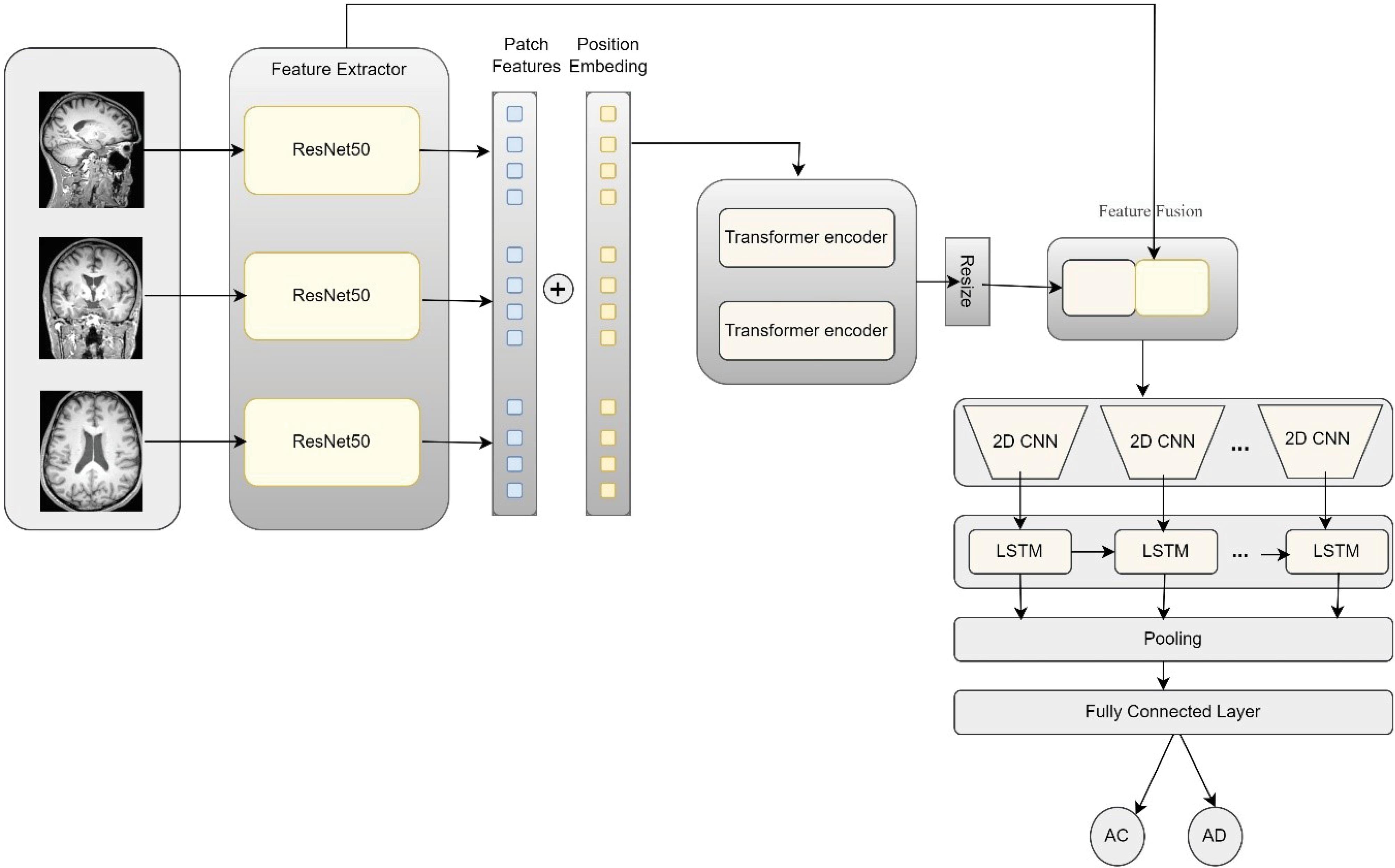
Fig. 1.
Overview of the proposed model and the details of its components.
.
Overview of the proposed model and the details of its components.
Feature extraction using ResNet
In the proposed method, three different views of the brain are utilized using MRI images: Sagittal (side view), Coronal (back view), and Axial (top view). Instead of using the Transformer alone as an encoder, this paper employs a CNN-Transformer combination. In this architecture, the CNN serves first as a feature extractor to generate feature maps. This approach is chosen for two main reasons: first, it allows us to utilize high-level features during the decoding process, and second, it offers better performance compared to using the Transformer alone.
To this end, each image X Î RC × H × W with resolution H × W and C channels is fed into the ResNet50 network, which extracts local and deep features from the images. In this study, the choice of ResNet50 as the primary model architecture was driven by its unique capabilities in extracting complex features from medical images, particularly MRI scans. Unlike architectures such as VGG, which can lead to overfitting and increased training time due to the high number of parameters and model complexity, ResNet50 leverages residual networks to capture both local and deep features while overcoming the vanishing gradient problem. Furthermore, ResNet50 is widely used in transfer learning, allowing us to benefit from its pretrained features to accelerate the feature extraction process. Additionally, when compared to other architectures like Efficient Net, ResNet50 has demonstrated superior performance in medical imaging tasks, particularly in brain disease detection from MRI images.
Additionally, by employing transfer learning, we can reduce the number of trainable parameters in the model. The output of this network for input data from each view is a tensor with dimensions 8 × 8 × d, where d = 2048 represents the number of feature channels.
(1)
Where XLi is the i-th MRI view (sagittal, coronal, or axial). Fi is the feature vector output from ResNet-50 for each view. Fig. 2 illustrates the overall architecture of the ResNet network. In this paper, we utilize the extracted features from different layers of the network in the subsequent stages. Therefore, the sizes of the generated images at each layer are indicated. For this purpose, the output from the last layer of this network, which contains 2048 distinct images of size 8 × 8, is used as inputs to the Transformer network. Additionally, to capture more detailed features, outputs from the preceding layers are also combined and transformed into feature vectors using pooling layers. These features are then integrated via skip connections with the features extracted from the Transformer network.
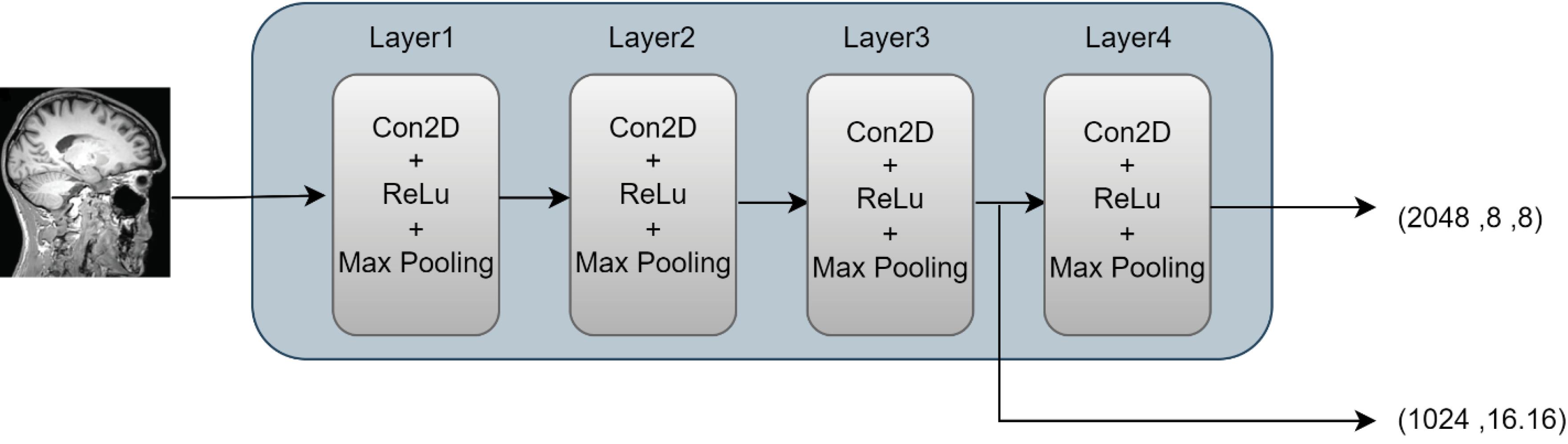
Fig. 2.
Architecture of ResNet used in the proposed method.
.
Architecture of ResNet used in the proposed method.
Feature extraction with the transformer network
The features extracted from the final layer of ResNet-50 are considered as patch features. Since the spatial arrangement of these patches is important, position embeddings are added to each patch to preserve their spatial order and positional information. This ensures that the model retains the contextual relationships between the patches during the subsequent processing stages.
By incorporating position embeddings, the Transformer can effectively understand the spatial context of the patch features, allowing for a more nuanced interpretation of the MRI data. This combination of feature extraction and positional information enhances the model’s ability to analyze and differentiate between various patterns within the brain images.
Here, Pi represents the position embedding for each patch. This step helps the model maintain the spatial relationships between the different image features. The local features, combined with the position embeddings, are fed as input to the Transformer encoder. The Transformer utilizes a self-attention mechanism to extract global features and relationships between different image patches. The attention mechanism is defined as follows:
(3)
In this context, Q, K, and V represent the query, key, and value matrices, respectively. The transformer encoder operates in several layers to extract the final features for each input. The Transformer Encoder module consists of Nencoder= 2 transformer layers. Each transformer layer comprises four sub-layers as follows: First sub-layer: Layer Norm, second sub-layer: Multi-Head Self-Attention, third sub-layer: Layer Norm, fourth sub-layer: Feedforward layer (MLP).
Feature fusion
After the high-level and global features are obtained through the transformer encoder, these features are combined with the local features extracted from ResNet. To do this, the output of the transformer is first resized so that its dimensions match those of the local features.
In this equation, Ffused represents the combined features obtained from the integration of global and local features. HiL is the output of the transformer for the i-th view of the MRI images. L indicates the last layer of the transformer encoder, which provides high-level (global) features. Resize(HiL) is the resizing operation that transforms the output of the transformer encoder into a matrix format. This combination allows the model to simultaneously capture detailed local information (details) and overall global context (structural elements) of the MRI images, which is crucial for improving the diagnosis of AD.
In the proposed method, a stack of Feature Fusion layers is used as the combiner. The Feature Fusion layer consists of four layers as follows: two ResUnits are embedded separately within this layer, one for the input features and the other for the skip connection. To increase the dimensions of the input features, they pass through an UpSampling layer after leaving the ResUnit. Additionally, to reduce the dimensions, a Conv1D operation is applied to decrease the number of input channels. Finally, the inputs are added together. The details of this phase are illustrated in Fig. 3.
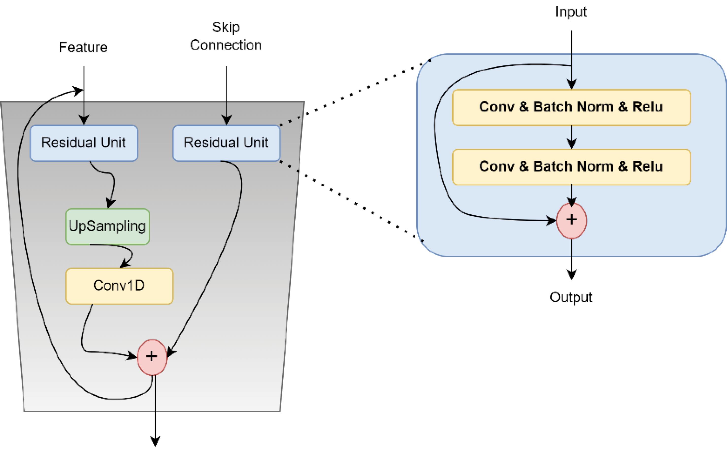
Fig. 3.
An overview of the architecture proposed for feature fusion.
.
An overview of the architecture proposed for feature fusion.
Classification module
After feature extraction using ResNet and Transformer networks and combining them, the classification module, which includes features from Con2D layers, LSTM, and fully connected layers, is used for data classification. To combine different features, 2D CNN layers are utilized.
To integrate the features between the CNN and LSTM layers, we first extract spatial features from the MRI images using the ResNet50-based CNN architecture. The CNN layers focus on capturing local spatial patterns in the data, such as texture and structure, which are crucial for detecting subtle differences in brain regions. These extracted features are then passed into the LSTM network, which captures temporal or sequential dependencies between the features across different perspectives (sagittal, coronal, and axial views). The LSTM layers allow the model to learn the relationships and changes in the features over different slices of the MRI, providing a dynamic representation of the data. This combination of CNN and LSTM facilitates the effective integration of both spatial and sequential information, crucial for accurate AD classification. In this stage, the final combined feature vectors are fed into multiple 2D CNN layers. These layers apply two-dimensional convolution operations on the data to extract higher-level and more complex features from the images. The convolution operation is defined as follows:
Where Oi is the output of the CNN layer and Ffused represents the input features. After extracting spatial features from the images using CNN, the outputs are fed into LSTM to model the sequential and temporal relationships between the images and their segments. LSTM is used for sequence modeling and is capable of effectively capturing time-dependent information. The general formula for LSTM is as follows:
In this formula, ht represents the hidden state at time t and Ot is the output of the CNN at time t. Finally, the features obtained from LSTM are fed into a pooling layer to reduce dimensions, and then into the fully connected layer. In this layer, the final classification for Alzheimer’s detection is performed using the Softmax function.
Model training
In this paper, we employ the Binary Cross-Entropy Loss function, which is suitable for binary classification problems. The loss function is defined as:
(7)
Where, N represents the number of samples, yi denotes the true label for the ith sample,
indicates the predicted probability that the ith sample belongs to the positive class.
To optimize the model, we implement the Adam Optimizer, an advanced optimization algorithm that combines the benefits of two other stochastic gradient descent extensions. Adam dynamically adjusts the learning rate for each parameter and employs moving averages of both the gradients and the squared gradients. The parameter update rule is expressed as follows:
Where, α is the learning rate, mt is the first moment estimate (the mean of the gradients), vt is the second moment estimate (the uncentered variance of the gradients), ϵ is a small constant to prevent division by zero. The first and second moments are updated according to:
gt represents the gradient of the loss function with respect to the model parameters at time step t, β1 and β2 are hyperparameters controlling the decay rates of the moment estimates. In the proposed method, the learning rate is set to lr = 1e−3, with β1 = 0.5 and β2 = 0.99, and mini-batches of size 32. To prevent overfitting and improve generalization, we employed the regularization technique of dropout, which randomly sets a portion of the input units to zero during training, ensuring the model does not become overly reliant on specific neurons. Additionally, to optimize the learning process and avoid overfitting, we used the Adam optimizer, which automatically adjusts the learning rate and performs efficient updates to the model's parameters, helping the model converge faster while maintaining robustness. The pseudocode of the proposed method is shown in Box 1.
Box 1. The pseudocode of the proposed method
Input: MRI slices (Axial, Coronal, Sagittal views)
1. Feature Extraction
2. Patch and Position Embedding
3. Transformer Encoding
4. Feature Fusion
5. 2D CNN + LSTM Sequence Modeling
6. Pooling
7. Fully Connected Layer
Output: Predicted class probabilities
Results
After training, this section evaluates the proposed method, which is based on multimodule and the transformer network and recurrent networks, by examining the model's performance using various evaluation metrics. The metrics used include accuracy, precision, ROC curve, and confusion matrix.
Dataset
This study focuses on identifying two main classes, namely AD and cognitively normal control groups (CN), using MRI image data from the ADNI database. Initially, a total of 47,825 scans were collected from various angles; however, to concentrate more on relevant anatomical information, only 10% of the middle slices from each scan were selected. This region was specifically chosen due to its provision of more meaningful information for distinguishing between the AD and CN classes. After this selection process, the final dataset consisted of 10,500 images for the AD class and 9300 images for the CN class.
To maintain balance and accuracy in the analysis, an equal number of images were chosen from each imaging angle. For instance, from the 9300 CN images, 3100 were selected from the sagittal view, 3100 from the axial view, and 3100 from the coronal view. The same approach was applied to the AD class as well. This careful selection aids in enhancing the accuracy of detection and analysis models.38
Evaluation metrics
In binary classification tasks, after classifying samples, four distinct outcomes can be observed. These outcomes are defined as follows:
-
True Negative (TN): The number of instances correctly classified as negative.
-
False Positive (FP): The number of instances incorrectly classified as positive.
-
True Positive (TP): The number of instances correctly classified as positive.
-
False Negative (FN): The number of instances incorrectly classified as negative.
To evaluate the effectiveness of classification methods, several metrics are used. Accuracy measures the proportion of correctly classified instances out of the total number of instances, calculated as:
(11)
Specificity indicates the percentage of true negatives correctly identified as such:
Sensitivity measures the percentage of true positives correctly identified:
Precision measures the accuracy of positive predictions. Specifically, it is the proportion of true positive instances among all instances classified as positive. This metric is particularly useful when the cost of false positives is high. Precision is calculated as:
A high precision value indicates that when the classifier predicts a positive outcome, it is likely to be correct.
The Matthews correlation coefficient (MCC) provides a comprehensive measure of a classifier's performance, taking into account true positives, true negatives, false positives, and false negatives. MCC is especially useful for imbalanced datasets because it considers all four confusion matrix categories. It is calculated as:
(15)
MCC returns a value between -1 and + 1, where:
+ 1 indicates a perfect classification.
0 indicates no better than random classification.
-1 indicates a total disagreement between prediction and observation.
MCC is a robust metric for binary classification, providing a balanced measure that is particularly informative in scenarios with class imbalance.38,39
Hyper-parameter tuning
The parameters selected in this research using the hyperparameter tuning technique, are the learning rate, optimizer, momentum, batch size, recurrent network type, and cache memory. The values provided for tuning the hyperparameters for the learning rate are 0.1, 0.01, 0.001, and 0.0001. Additionally, the values given for the cache memory are 16, 64, and 128. Table 1 shows the hyperparameters used in the proposed method.
Table 1.
Investigating the amount of hyperparameters used in the proposed method
|
Hyperparameter
|
Tested values
|
Chosen value
|
| Loss function |
CrossEntropyLoss |
CrossEntropyLoss |
| Optimizer |
SGD, Adam |
Adam |
| Momentum |
1e-6, 1e-5,1e-4,1e-3 |
1e-6 |
| Learning rate |
0.1, 0.01,0.001,0.0001 |
0.001 |
| Batch size |
16,32,64 |
32 |
| Hidden state |
16,32,64,128 |
64 |
| Recurrent network |
LSTM, GRU, RNN |
LSTM |
These values were obtained based on various experiments. For this purpose, 500 images from the dataset were randomly selected from two classes. Then, the model was trained using these data based on the best configuration of each hyperparameter. For example, the learning rate was tested with different values, and the best value was found to be 0.01. Then, with this hyperparameter fixed, the momentum value was calculated.
Initially, given the importance of recurrent layers in the proposed method, the models were tested with different layers. These layers include LSTM, GRU, and recurrent neural network (RNN). The results of these experiments on the test data, based on accuracy, precision, and other metrics, are presented in Table 2. It is noteworthy that in all experiments, the cache memory and the number of iterations for training the models were set to 16 and 100, respectively.
Table 2.
Results of the proposed method based on various metrics using different recurrent networks
|
Eval metric Model
|
Data
|
Accuracy
|
Precision
|
Recall
|
F1 score
|
ROC curve
|
| RNN |
Train |
1 |
0.999 |
1 |
0.999 |
0.9973 |
| Validation |
0.963 |
0.967 |
0.962 |
0.964 |
0.9843 |
| Test |
0.946 |
0.9481 |
0.9432 |
0.9451 |
0.9720 |
| LSTM |
Train |
1 |
0.998 |
1 |
1 |
0.9994 |
| Validation |
0.9812 |
0.986 |
0.981 |
0.982 |
0.9941 |
| Test |
0.9692 |
0.9636 |
0.9625 |
0.9634 |
0988 |
| GRU |
Train |
1 |
1 |
1 |
1 |
0.9999 |
| Validation |
0.977 |
0.976 |
0.972 |
0.97 |
0.9896 |
| Test |
0.9508 |
0.9516 |
0.9577 |
0.9593 |
0.9812 |
As shown in the results of the table, a 100% accuracy rate was reported on the training dataset, and other metrics also performed at a high level. Importantly, there is not a significant numerical gap between the various metrics, indicating that the proposed method has effectively learned the features of both classes. Furthermore, all three recurrent networks demonstrate a high detection rate, suggesting that the proposed method is not heavily dependent on the type of recurrent network. However, among the three recurrent networks, the GRU network has the highest detection rate.
Convergence Process
Given that the proposed method has a large number of parameters, learning these parameters can be challenging. To evaluate the learning process of the proposed method, the error and accuracy charts of the training and evaluation datasets are presented in Fig. 4. As shown in Fig. 4, the error rate in both the training and evaluation sets for various recurrent networks has decreased. Although the gap between the error charts in the training and evaluation sets is large, this does not indicate overfitting of the proposed model; because, in different iterations, this error gap does not increase and the error remains at a constant level.
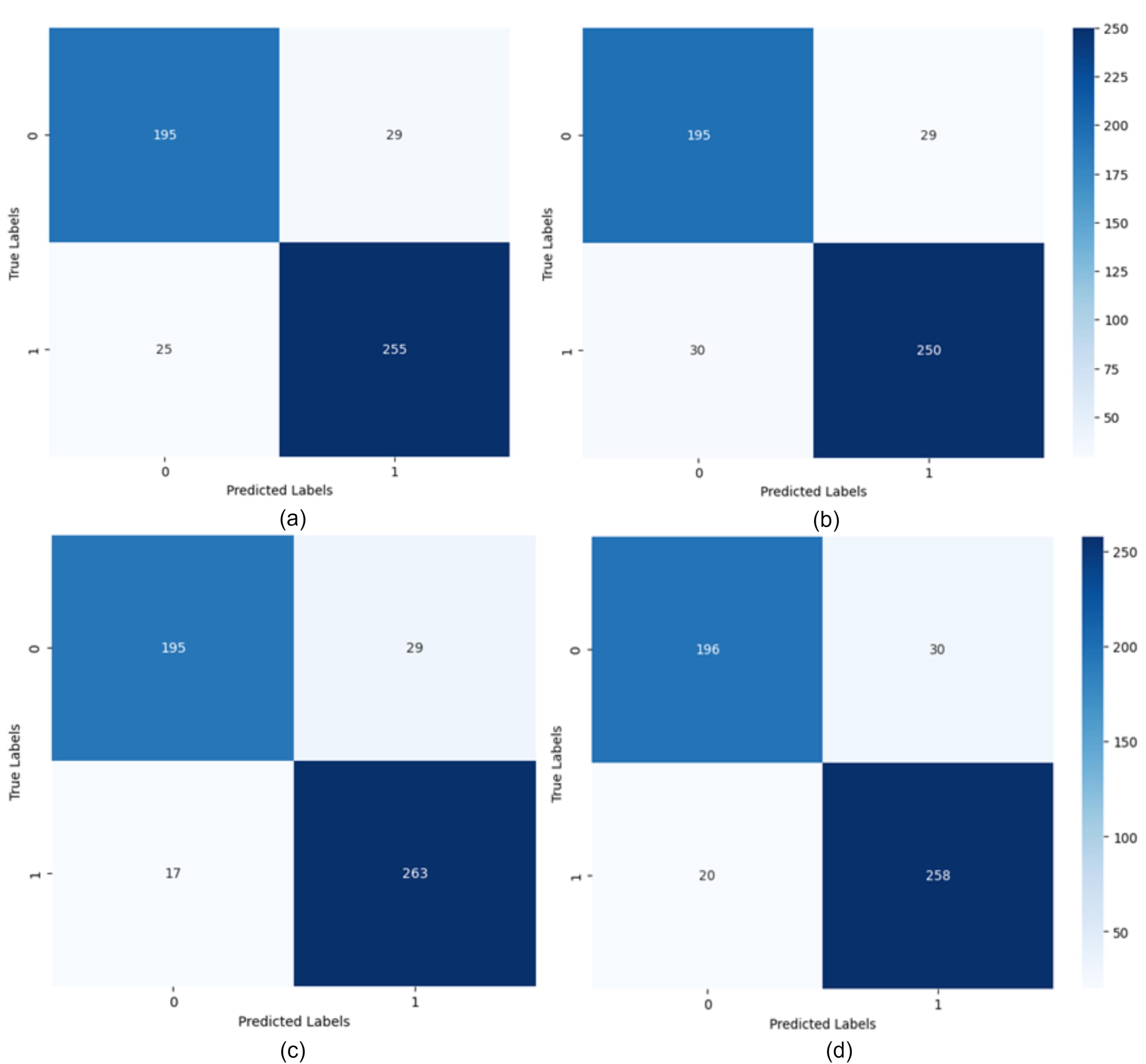
Fig. 4.
Confusion matrix for LSTM networks with different hidden state lengths: a) Hidden state vector length 16, b) Hidden state vector length 32, c) Hidden state vector length 64, d) Hidden state vector length 128.
.
Confusion matrix for LSTM networks with different hidden state lengths: a) Hidden state vector length 16, b) Hidden state vector length 32, c) Hidden state vector length 64, d) Hidden state vector length 128.
Additionally, considering the accuracy chart of the training and evaluation datasets shown in Fig. 5, it can be seen that the learning process is proceeding correctly. The model’s accuracy gradually increases and, after a certain point, the model’s accuracy remains stable and does not decrease. This indicates that the model has reached a stable level of learning and provides satisfactory performance in data separation.
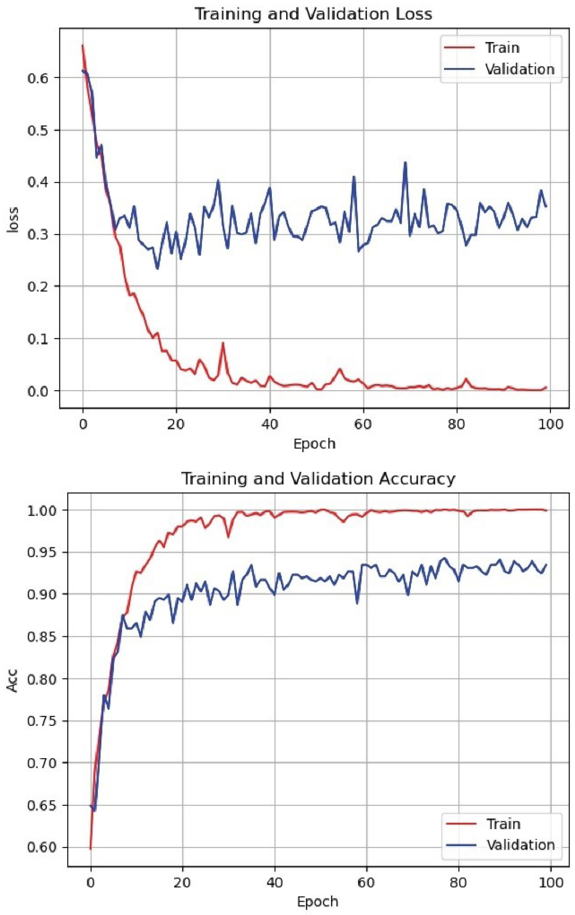
Fig. 5.
Loss function and accuracy of the proposed method on training and evaluation dataset.
.
Loss function and accuracy of the proposed method on training and evaluation dataset.
Batch size is one of the most important parameters in deep learning models, referring to the number of samples the model processes in each step. The batch size analysis in the proposed method was conducted using batch sizes of 16, 32, 64, and 128. The experiment was carried out over 10 epochs, with 80% of the data used for training. The learning rate was kept constant at 0.001 for all cases. The results showed that a batch size of 32 provided the best performance with an accuracy of 96.92%. The accuracies achieved for batch sizes 128, 64, and 16 were 93.21%, 94.72%, and 94.23%, respectively. Using a confusion matrix is suitable for better evaluating the proposed method and examining the model’s ability to predict different classes. In Fig. 4, the confusion matrices resulting from training the model with different hidden state sizes and iterations, trained using LSTM, are shown. As observed, with 100 iterations and a hidden state vector length of 64, the RNN performs best.
Additionally, to evaluate the performance of different recurrent networks, Fig. 6 shows the confusion matrices of three models: LSTM, GRU, and RNN, with the same number of iterations and hidden states. In this experiment, the hidden state vector length, number of iterations, and other parameters such as learning rate and activation function are set the same for all three networks. As observed, all recurrent networks have suitable performance, indicating that the combined features are independent of the type of recurrent network. Moreover, among these three networks, GRU shows better performance due to having fewer parameters compared to LSTM and greater capability compared to RNN.
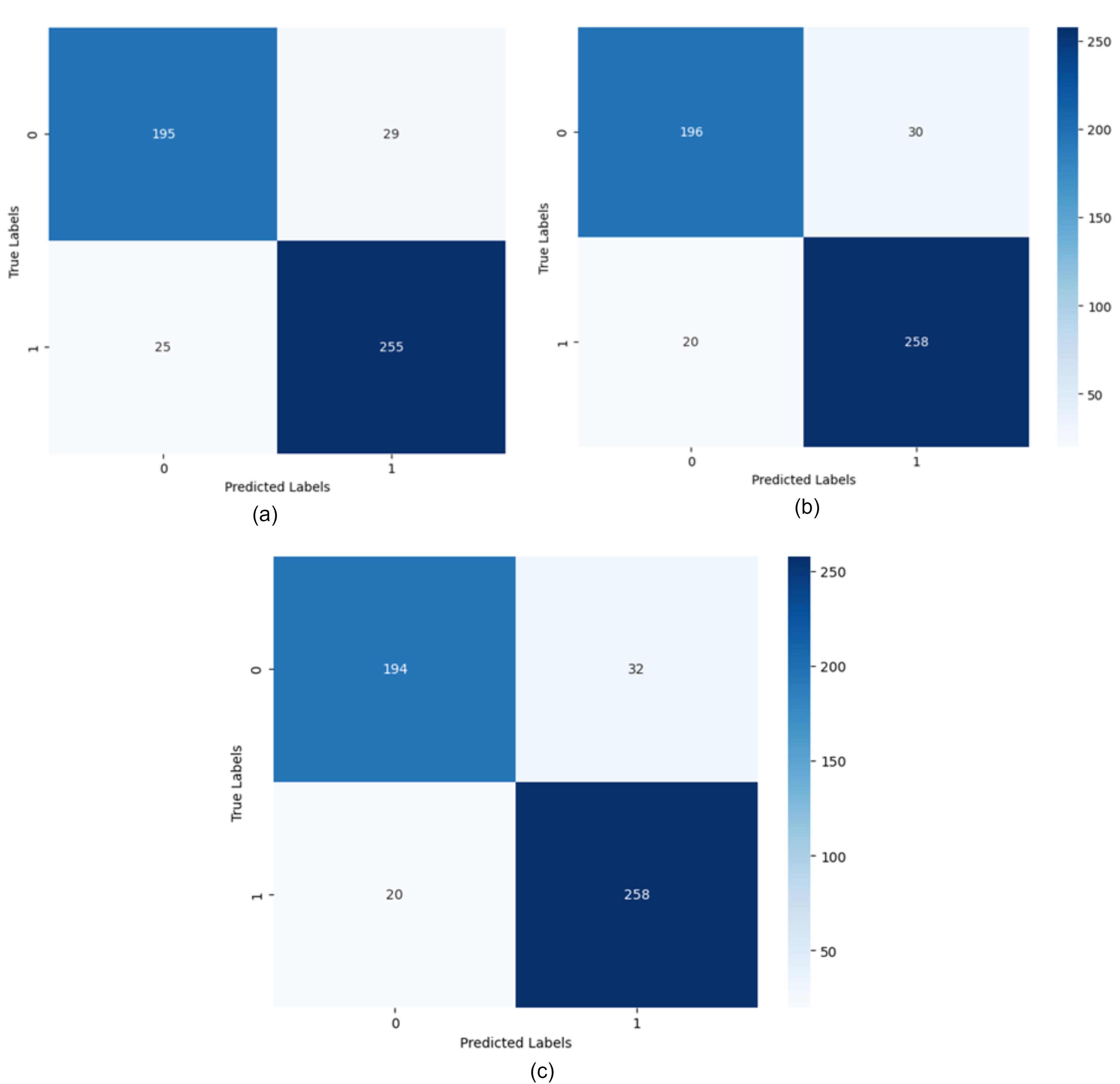
Fig. 6.
The confusion matrix for different recurrent networks with a hidden state length of 16 (a) LSTM recurrent network, (b) GRU recurrent network, (c) RNN recurrent network.
.
The confusion matrix for different recurrent networks with a hidden state length of 16 (a) LSTM recurrent network, (b) GRU recurrent network, (c) RNN recurrent network.
Given the imbalance of data in the two classes, Figs. 7 and 8 show the ROC and PR curves for the proposed method. The PR curve, which stands for Precision and Recall, is a two-dimensional chart that shows precision and recall at each iteration. Additionally, the ROC curve is a graphical chart that displays the performance of a binary classification model by plotting the true positive rate (sensitivity) against the false positive rate (1-specificity) at various threshold settings.
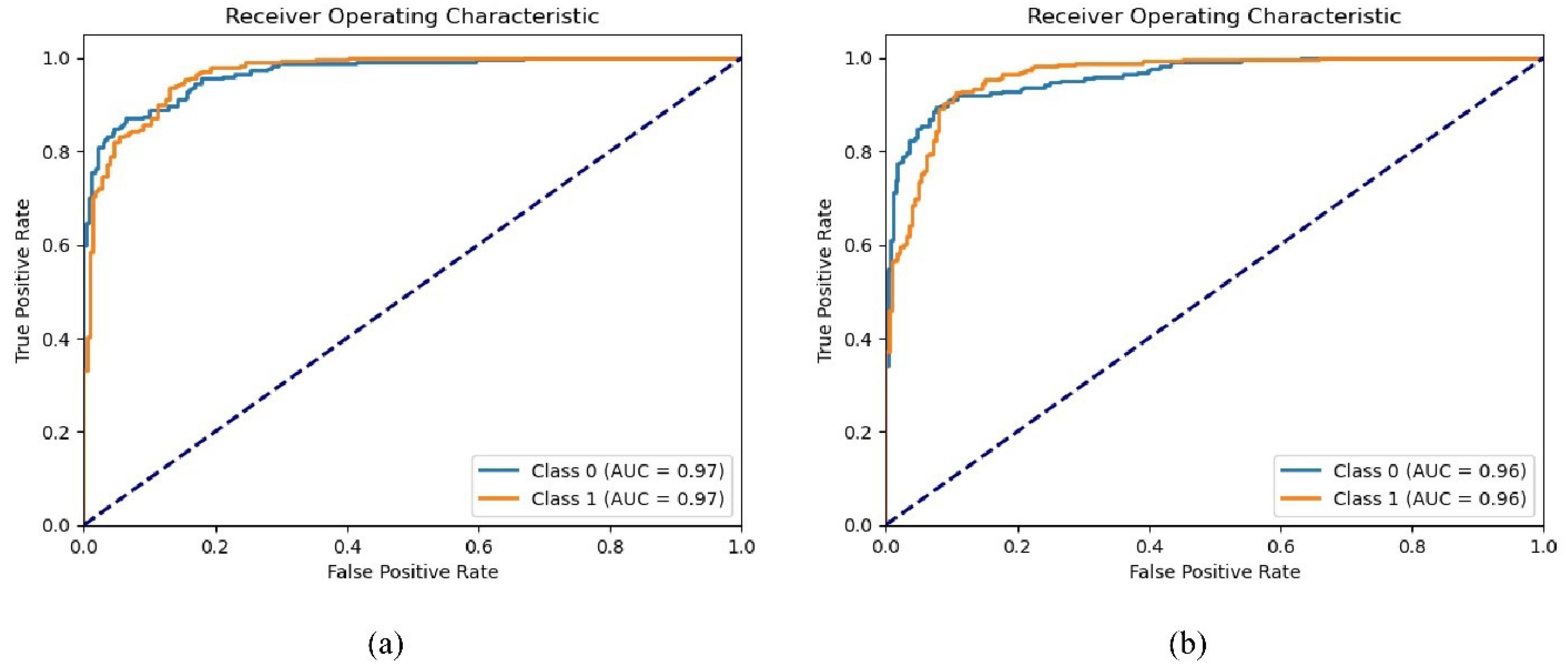
Fig. 7.
ROC curve on the test dataset for two classes based on different recurrent models. a) LSTM recurrent network, b) GRU recurrent network.
.
ROC curve on the test dataset for two classes based on different recurrent models. a) LSTM recurrent network, b) GRU recurrent network.
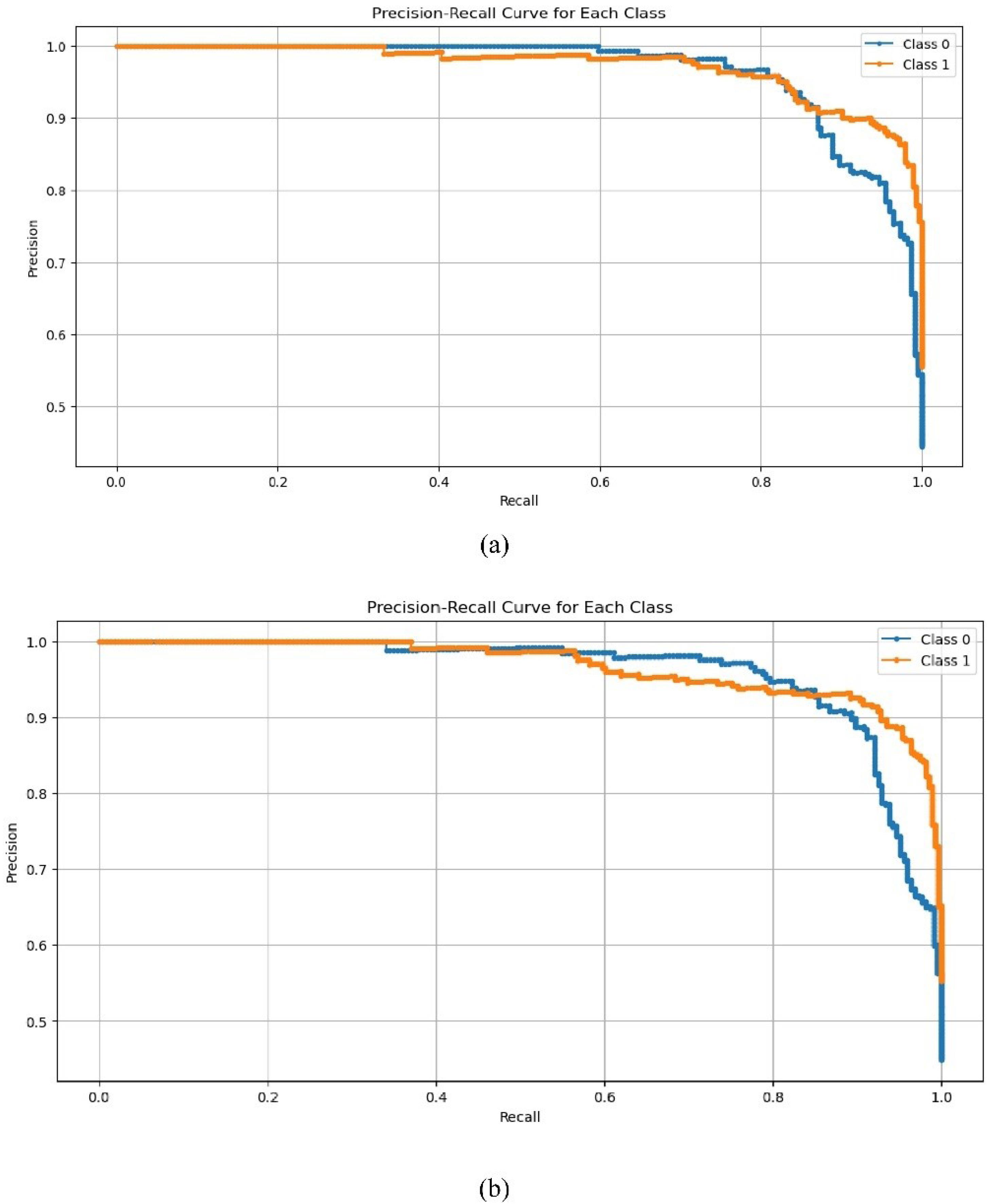
Fig. 8.
PR curve on the test dataset for two classes based on different recurrent models. a) LSTM recurrent network, b) GRU recurrent network.
.
PR curve on the test dataset for two classes based on different recurrent models. a) LSTM recurrent network, b) GRU recurrent network.
Comparison with other methods
The evaluation and comparison of the proposed method with other methods have been examined based on the accuracy criterion. The results of this experiment are presented in Table 3. Since there is no uniform and standard dataset for testing different models, the methods selected for this comparison have all been published in recent years and have used the ADNI dataset for image collection. Additionally, deep learning-based methods have been selected.
Table 3.
Comparison of the proposed method with other methods
|
Method
|
Year
|
Data
|
Participants
|
Accuracy
|
| Multimodal42 |
2024 |
EEG + SNP + PRS |
270 |
86.2 |
| ResNet 43 |
2020 |
MRI |
394 |
89.3 |
| Lasso 44 |
2021 |
MRI + PET |
302 |
84.7 |
| CNN 45 |
2020 |
MRI |
2490 |
82.4 |
| CNN 46 |
2020 |
PET |
479 |
83.0 |
| PCA Net 3D ShuffleNet 47 |
2021 |
MRI |
2450 |
85.2 |
| VGG16, ResNet 50 and modified AlexNet 28 |
2021 |
MRI |
22300 |
95.70 |
| VGG 48 |
2022 |
MRI |
21000 |
95.89 |
| Proposed method |
2024 |
MRI |
19800 |
96.92 |
The results indicate that the proposed method outperforms many existing approaches, with the exception of VGG-based methods, which demonstrate comparable performance. However, the primary distinction lies in the number of images utilized; the VGG-based methods employ a significantly larger dataset than our proposed approach. Furthermore, methods based on VGG16 and the modified version of AlexNet exhibit much longer execution times. While these methods independently achieve detection rates ranging from 82% to 95%, our proposed method consistently demonstrates 1% to 14% better performance compared to other methods.
Computational cost analysis
The execution time of the proposed method is influenced by several factors, including the use of ResNet50 for feature extraction, the Transformer encoder for high-level feature extraction, and the LSTM layers for sequence modeling. While the ResNet50 model significantly reduces the number of trainable parameters through transfer learning, the inclusion of the Transformer and LSTM layers introduces additional computational complexity. The Transformer encoder, with its multi-head self-attention mechanism, requires substantial processing power, especially when handling the high-dimensional feature maps from the ResNet network. Furthermore, LSTM layers, though efficient at capturing sequential dependencies, increase the computational load due to their recurrent nature, which processes the data step-by-step.
Despite these complexities, our model achieves a reasonable balance between accuracy and execution time. We observed that, although the model's execution time is longer compared to simpler architectures, the inclusion of these advanced modules results in improved classification performance, which justifies the additional computational cost. Additionally, optimizations such as the use of pre-trained networks, the Adam optimizer for efficient training, and regularization techniques like dropout help manage the computational burden and reduce the risk of overfitting, making the model practical for real-world applications in medical diagnostics.
The time complexity of the proposed method can be analyzed by considering the main components of the architecture: ResNet50, the Transformer encoder, and the LSTM layers.
ResNet50: The time complexity of feature extraction using ResNet50 is dominated by the convolutional layers. Since ResNet50 consists of several convolutional layers and residual blocks, the time complexity for processing an input image can be approximated as O(n × m × C × H × W), where n is the number of input images, m is the number of layers, C is the number of channels, and H and W are the height and width of the input image.
Transformer Encoder: The Transformer encoder applies multi-head self-attention, which has a time complexity of O(N^2 × d), where N is the number of input patches (corresponding to the number of features after the ResNet extraction) and d is the dimensionality of the feature space. The self-attention mechanism requires comparing each patch with every other patch, leading to the quadratic dependency on the number of patches.
LSTM: The time complexity of the LSTM layer is O(T × d), where T is the length of the sequence (number of MRI slices or views) and d is the dimensionality of the feature vector at each time step. Since the LSTM processes the data sequentially, it introduces a linear complexity with respect to the sequence length.
Overall, the time complexity of the entire model is dominated by the Transformer encoder due to its quadratic dependency on the number of patches. Therefore, the overall time complexity can be approximated as O(N^2 × d + T × d), where N is the number of patches from the ResNet output, d is the feature dimensionality, and T is the sequence length for the LSTM layers. This suggests that the execution time grows quadratically with the number of input patches but linearly with respect to the sequence length in the LSTM module.
Conclusion
In this article, we propose a Multimodal approach to feature extraction from MRI images for diagnosing AD. By utilizing images from sagittal, coronal, and axial views, we first employ ResNet50 for effective local feature extraction. This is followed by a Transformer encoder that integrates positional embeddings to maintain spatial relationships, enabling nuanced interpretations of the MRI data. The resulting feature vectors are fused to retain both high-level and detailed information. For classification, we incorporate 2D CNN and LSTM layers to address the sequential nature of the data, culminating in a fully connected layer that uses the Softmax function for final classification. Our method demonstrates superior performance on the ADNI dataset, achieving high accuracy rates of 96.92% on test data and 98.12% on validation data.
The proposed method successfully combines the strengths of CNN and Transformer architectures, significantly enhancing feature extraction and classification accuracy. By leveraging transfer learning and employing a multi-view approach, we improve the model's ability to discern complex patterns within MRI data. The results indicate that our framework not only serves as a reliable diagnostic tool but also sets a benchmark for future research in this area. The achieved accuracy rates represent a substantial advancement over existing methodologies, paving the way for more effective early diagnosis and intervention strategies for AD.
Research Highlights
What is the current knowledge?
What is new here?
Competing Interests
Authors declare no conflict of interests.
Ethical Approval
Not applicable.
References
- Viswan V, Shaffi N, Mahmud M, Subramanian K, Hajamohideen F. Explainable artificial intelligence in Alzheimer’s disease classification: a systematic review. Cognit Comput 2024; 16:1-44. doi: 10.1007/s12559-023-10192-x [Crossref] [ Google Scholar]
- Odusami M, Maskeliūnas R, Damaševičius R, Misra S. Machine learning with multimodal neuroimaging data to classify stages of Alzheimer's disease: a systematic review and meta-analysis. CognNeurodyn 2024; 18:775-94. doi: 10.1007/s11571-023-09993-5 [Crossref] [ Google Scholar]
- Hcini G, Jdey I, Dhahri H. Investigating deep learning for early detection and decision-making in Alzheimer’s disease: a comprehensive review. Neural Process Lett 2024; 56:153. doi: 10.1007/s11063-024-11600-5 [Crossref] [ Google Scholar]
- Suganyadevi S, Pershiya AS, Balasamy K, Seethalakshmi V, Bala S, Arora K. Deep learning-based Alzheimer disease diagnosis: a comprehensive review. SN Comput Sci 2024; 5:391. doi: 10.1007/s42979-024-02743-2 [Crossref] [ Google Scholar]
- Arya AD, Verma SS, Chakarabarti P, Chakrabarti T, Elngar AA, Kamali AM. A systematic review on machine learning and deep learning techniques in the effective diagnosis of Alzheimer's disease. Brain Inform 2023; 10:17. doi: 10.1186/s40708-023-00195-7 [Crossref] [ Google Scholar]
- Garg N, Choudhry MS, Bodade RM. A review on Alzheimer's disease classification from normal controls and mild cognitive impairment using structural MR images. J Neurosci Methods 2023; 384:109745. doi: 10.1016/j.jneumeth.2022.109745 [Crossref] [ Google Scholar]
- Zhou Q, Wang J, Yu X, Wang S, Zhang Y. A survey of deep learning for Alzheimer’s disease. Mach Learn KnowlExtr 2023; 5:611-68. doi: 10.3390/make5020035 [Crossref] [ Google Scholar]
- Rao BS, Aparna M. A review on Alzheimer’s disease through analysis of MRI images using deep learning techniques. IEEE Access 2023; 11:71542-56. doi: 10.1109/access.2023.3294981 [Crossref] [ Google Scholar]
- Illakiya T, Karthik R. Automatic detection of Alzheimer's disease using deep learning models and neuro-imaging: current trends and future perspectives. Neuroinformatics 2023; 21:339-64. doi: 10.1007/s12021-023-09625-7 [Crossref] [ Google Scholar]
- Zhao Y, Guo Q, Zhang Y, Zheng J, Yang Y, Du X. Application of deep learning for prediction of Alzheimer's disease in PET/MR imaging. Bioengineering (Basel) 2023; 10:1120. doi: 10.3390/bioengineering10101120 [Crossref] [ Google Scholar]
- Alatrany AS, Khan W, Hussain A, Kolivand H, Al-Jumeily D. An explainable machine learning approach for Alzheimer's disease classification. Sci Rep 2024; 14:2637. doi: 10.1038/s41598-024-51985-w [Crossref] [ Google Scholar]
- Liu X, Tosun D, Weiner MW, Schuff N. Locally linear embedding (LLE) for MRI based Alzheimer's disease classification. Neuroimage 2013; 83:148-57. doi: 10.1016/j.neuroimage.2013.06.033 [Crossref] [ Google Scholar]
- Altaf T, Anwar SM, Gul N, Majeed MN, Majid M. Multi-class Alzheimer's disease classification using image and clinical features. Biomed Signal Process Control 2018; 43:64-74. doi: 10.1016/j.bspc.2018.02.019 [Crossref] [ Google Scholar]
- Alam S, Kwon GR. Alzheimer disease classification using KPCA, LDA, and multi-kernel learning SVM. Int J Imaging Syst Technol 2017; 27:133-43. doi: 10.1002/ima.22217 [Crossref] [ Google Scholar]
- Diogo VS, Ferreira HA, Prata D. Early diagnosis of Alzheimer's disease using machine learning: a multi-diagnostic, generalizable approach. Alzheimers Res Ther 2022; 14:107. doi: 10.1186/s13195-022-01047-y [Crossref] [ Google Scholar]
- Tripathi T, Kumar R. Speech-based detection of multi-class Alzheimer’s disease classification using machine learning. Int J Data Sci Anal 2024; 18:83-96. doi: 10.1007/s41060-023-00475-9 [Crossref] [ Google Scholar]
- Al Shehri W. Alzheimer's disease diagnosis and classification using deep learning techniques. PeerJComput Sci 2022; 8:e1177. doi: 10.7717/peerj-cs.1177 [Crossref] [ Google Scholar]
- Qiu S, Joshi PS, Miller MI, Xue C, Zhou X, Karjadi C. Development and validation of an interpretable deep learning framework for Alzheimer's disease classification. Brain 2020; 143:1920-33. doi: 10.1093/brain/awaa137 [Crossref] [ Google Scholar]
- Chen Y, Wang L, Ding B, Shi J, Wen T, Huang J. Automated Alzheimer's disease classification using deep learning models with Soft-NMS and improved ResNet50 integration. J Radiat Res Appl Sci 2024; 17:100782. doi: 10.1016/j.jrras.2023.100782 [Crossref] [ Google Scholar]
- Zhang J, Zheng B, Gao A, Feng X, Liang D, Long X. A 3D densely connected convolution neural network with connection-wise attention mechanism for Alzheimer's disease classification. MagnReson Imaging 2021; 78:119-26. doi: 10.1016/j.mri.2021.02.001 [Crossref] [ Google Scholar]
- Ebrahimi A, Luo S. Convolutional neural networks for Alzheimer's disease detection on MRI images. J Med Imaging (Bellingham) 2021; 8:024503. doi: 10.1117/1.Jmi.8.2.024503 [Crossref] [ Google Scholar]
- Samhan LF, Alfarra AH, Abu-Naser SS. Classification of Alzheimer's disease using convolutional neural networks. Int J Acad Inform Syst Res 2022; 6:18-23. [ Google Scholar]
- Jain R, Jain N, Aggarwal A, Hemanth DJ. Convolutional neural network-based Alzheimer’s disease classification from magnetic resonance brain images. Cogn Syst Res 2019; 57:147-59. doi: 10.1016/j.cogsys.2018.12.015 [Crossref] [ Google Scholar]
- Salehi AW, Baglat P, Sharma BB, Gupta G, Upadhya A. A CNN model: earlier diagnosis and classification of Alzheimer disease using MRI. In: 2020 International Conference on Smart Electronics and Communication (ICOSEC). Trichy, India: IEEE; 2020. p. 156-61. doi: 10.1109/icosec49089.2020.9215402.
- Long X, Chen L, Jiang C, Zhang L. Prediction and classification of Alzheimer disease based on quantification of MRI deformation. PLoS One 2017; 12:e0173372. doi: 10.1371/journal.pone.0173372 [Crossref] [ Google Scholar]
-
Mehmood A, Maqsood M, Bashir M, Shuyuan Y. A deep Siamese convolution neural network for multi-class classification of Alzheimer disease. Brain Sci 2020; 10. doi: 10.3390/brainsci10020084.
-
Aderghal K, Khvostikov A, Krylov A, Benois-Pineau J, Afdel K, Catheline G. Classification of Alzheimer disease on imaging modalities with deep CNNs using cross-modal transfer learning. In: 2018 IEEE 31st International Symposium on Computer-Based Medical Systems (CBMS). Karlstad, Sweden: IEEE; 2018. p. 345-50. doi: 10.1109/cbms.2018.00067.
-
Acharya H, Mehta R, Singh DK. Alzheimer disease classification using transfer learning. In: 2021 5th International Conference on Computing Methodologies and Communication (ICCMC). Erode, India: IEEE; 2021. p. 1503-8. doi: 10.1109/iccmc51019.2021.9418294.
- Tanveer M, Rashid AH, Ganaie MA, Reza M, Razzak I, Hua KL. Classification of Alzheimer's disease using ensemble of deep neural networks trained through transfer learning. IEEE J Biomed Health Inform 2022; 26:1453-63. doi: 10.1109/jbhi.2021.3083274 [Crossref] [ Google Scholar]
- Lella E, Pazienza A, Lofu D, Anglani R, Vitulano F. An ensemble learning approach based on diffusion tensor imaging measures for Alzheimer’s disease classification. Electronics 2021; 10:249. doi: 10.3390/electronics10030249 [Crossref] [ Google Scholar]
- Rajesh Khanna M. Multi-level classification of Alzheimer disease using DCNN and ensemble deep learning techniques. Signal Image Video Process 2023; 17:3603-11. doi: 10.1007/s11760-023-02586-z [Crossref] [ Google Scholar]
- Chatterjee S, Byun YC. Voting ensemble approach for enhancing Alzheimer's disease classification. Sensors (Basel) 2022; 22:7661. doi: 10.3390/s22197661 [Crossref] [ Google Scholar]
- Alp S, Akan T, Bhuiyan MS, Disbrow EA, Conrad SA, Vanchiere JA. Joint transformer architecture in brain 3D MRI classification: its application in Alzheimer's disease classification. Sci Rep 2024; 14:8996. doi: 10.1038/s41598-024-59578-3 [Crossref] [ Google Scholar]
-
Zhang L, Wang L, Zhu D. Jointly analyzing Alzheimer's disease related structure-function using deep cross-model attention network. In: 2020 IEEE 17th International Symposium on Biomedical Imaging (ISBI). Iowa City, IA: IEEE; 2020. p. 563-7. doi: 10.1109/isbi45749.2020.9098638.
-
Xing X, Liang G, Zhang Y, Khanal S, Lin AL, Jacobs N. Advit: vision transformer on multi-modality pet images for Alzheimer disease diagnosis. In: 2022 IEEE 19th International Symposium on Biomedical Imaging (ISBI). Kolkata, India: IEEE; 2022. p. 1-4. doi: 10.1109/isbi52829.2022.9761584.
- Liu L, Liu S, Zhang L, To XV, Nasrallah F, Chandra SS. Cascaded multi-modal mixing transformers for Alzheimer's disease classification with incomplete data. Neuroimage 2023; 277:120267. doi: 10.1016/j.neuroimage.2023.120267 [Crossref] [ Google Scholar]
-
Li C, Cui Y, Luo N, Liu Y, Bourgeat P, Fripp J, et al. Trans-ResNet: integrating transformers and CNNs for Alzheimer’s disease classification. In: 2022 IEEE 19th International Symposium on Biomedical Imaging (ISBI). Kolkata, India: IEEE; 2022. p. 1-5. doi: 10.1109/isbi52829.2022.9761549.
- Hu Z, Li Y, Wang Z, Zhang S, Hou W. Conv-Swinformer: integration of CNN and shift window attention for Alzheimer's disease classification. Comput Biol Med 2023; 164:107304. doi: 10.1016/j.compbiomed.2023.107304 [Crossref] [ Google Scholar]
- Alzheimer’s Disease Neuroimaging Initiative (ADNI). Available from: http://adni.loni.usc.edu.
- Sokolova M, Lapalme G. A systematic analysis of performance measures for classification tasks. Inf Process Manag 2009; 45:427-37. doi: 10.1016/j.ipm.2009.03.002 [Crossref] [ Google Scholar]
-
Davis J, Goadrich M. The relationship between precision-recall and ROC curves. In: Proceedings of the 23rd International Conference on Machine Learning. New York, NY: Association for Computing Machinery; 2006. p. 233-40. doi: 10.1145/1143844.1143874.
- Yu WY, Sun TH, Hsu KC, Wang CC, Chien SY, Tsai CH. Comparative analysis of machine learning algorithms for Alzheimer's disease classification using EEG signals and genetic information. Comput Biol Med 2024; 176:108621. doi: 10.1016/j.compbiomed.2024.108621 [Crossref] [ Google Scholar]
- Abrol A, Bhattarai M, Fedorov A, Du Y, Plis S, Calhoun V. Deep residual learning for neuroimaging: an application to predict progression to Alzheimer's disease. J Neurosci Methods 2020; 339:108701. doi: 10.1016/j.jneumeth.2020.108701 [Crossref] [ Google Scholar]
- Lin W, Gao Q, Yuan J, Chen Z, Feng C, Chen W. Predicting Alzheimer's disease conversion from mild cognitive impairment using an extreme learning machine-based grading method with multimodal data. Front Aging Neurosci 2020; 12:77. doi: 10.3389/fnagi.2020.00077 [Crossref] [ Google Scholar]
- Bae J, Stocks J, Heywood A, Jung Y, Jenkins L, Hill V. Transfer learning for predicting conversion from mild cognitive impairment to dementia of Alzheimer's type based on a three-dimensional convolutional neural network. Neurobiol Aging 2021; 99:53-64. doi: 10.1016/j.neurobiolaging.2020.12.005 [Crossref] [ Google Scholar]
- Pan X, Phan TL, Adel M, Fossati C, Gaidon T, Wojak J. Multi-view separable pyramid network for AD prediction at MCI stage by 18F-FDG brain PET imaging. IEEE Trans Med Imaging 2021; 40:81-92. doi: 10.1109/tmi.2020.3022591 [Crossref] [ Google Scholar]
- Odusami M, Maskeliūnas R, Damaševičius R, Krilavičius T. Analysis of features of Alzheimer's disease: detection of early stage from functional brain changes in magnetic resonance images using a finetuned ResNet18 network. Diagnostics (Basel) 2021; 11:1071. doi: 10.3390/diagnostics11061071 [Crossref] [ Google Scholar]
- Naz S, Ashraf A, Zaib A. Transfer learning using freeze features for Alzheimer neurological disorder detection using ADNI dataset. Multimed Syst 2022; 28:85-94. doi: 10.1007/s00530-021-00797-3 [Crossref] [ Google Scholar]