Bioimpacts. 2025;15:30468.
doi: 10.34172/bi.30468
Original Article
Predicting drug protein interactions based on improved support vector data description in unbalanced data
Alireza Khorramfard Formal analysis, Investigation, Methodology, Resources, Software, Validation, Visualization, Writing – original draft, Writing – review & editing, 
Jamshid Pirgazi Conceptualization, Data curation, Formal analysis, Investigation, Project administration, Resources, Supervision, Writing – review & editing, , *
Ali Ghanbari Sorkhi Data curation, Formal analysis, Investigation, Supervision, Visualization, Writing – review & editing,
Author information:
Department of Electrical and Computer Engineering, University of Science and Technology of Mazandaran, Behshahr, Iran
Abstract
Introduction:
Predicting drug-protein interactions is critical in drug discovery, but traditional laboratory methods are expensive and time-consuming. Computational approaches, especially those leveraging machine learning, are increasingly popular. This paper introduces VASVDD, a multi-step method to predict drug-protein interactions. First, it extracts features from amino acid sequences in proteins and drug structures. To address the challenge of unbalanced datasets, a Support Vector Data Description (SVDD) approach is employed, outperforming standard techniques like SMOTE and ENN in balancing data. Subsequently, dimensionality reduction using a Variational Autoencoder (VAE) reduces features from 1074 to 32, improving computational efficiency and predictive performance.
Methods:
The proposed method was evaluated on four datasets related to enzymes, G-protein-coupled receptors, ion channels, and nuclear receptors. Without preprocessing, the Gradient Boosting Classifier showed bias towards the majority class. However, balancing and dimensionality reduction significantly improved accuracy, sensitivity, specificity, and F1 scores. VASVDD demonstrated superior performance compared to other dimensionality reduction methods, such as kernel principal component analysis (kernel PCA) and Principal Component Analysis (PCA), and was validated across multiple classifiers, achieving higher AUROC values than existing techniques.
Results:
The results highlight VASVDD's effectiveness and generalizability in predicting drug-target interactions. The method outperforms state-of-the-art techniques in terms of accuracy, robustness, and efficiency, making it a promising tool in bioinformatics for drug discovery.
Conclusion:
The datasets analyzed during the current study are not publicly available but are available from the corresponding author upon reasonable request and source code are available on GitHub: https://github.com/alirezakhorramfard/vasvdd.
Keywords: Drug-protein interaction, Support vector data, Deep learning, Variational autoencoder, Unbalanced data
Copyright and License Information
© 2025 The Author(s).
This work is published by BioImpacts as an open access article distributed under the terms of the Creative Commons Attribution Non-Commercial License (
http://creativecommons.org/licenses/by-nc/4.0/). Non-commercial uses of the work are permitted, provided the original work is properly cited.
Funding Statement
Not applicable.
Introduction
The development of molecular medicine and the completion of the Human Genome Project have significantly enhanced opportunities to identify new target proteins for drug development.1 Traditional methods for exploring drug target interactions (DTIs) have been costly and time-consuming.2 Therefore, predicting DTIs has become crucial in pharmaceutical science to streamline drug candidate screening and address related issues. Improved biochemical technologies have accelerated drug discovery; however, the FDA has recently approved only a limited number of drugs due to efficacy and safety concerns.3 Advances in protein sequencing, drug molecular structure determination, and the availability of diverse databases have motivated the development of computational approaches for detecting potential interactions.4 These databases provide valuable experimental interaction data for developing new computational methods for large-scale DTI prediction.
Computational methods for predicting DTIs can be categorized into ligand-based, docking-based, and chemogenomic approaches. Ligand-based methods,5 such as quantitative structure-activity relationship (QSAR),6 predict interactions by comparing new ligands to known protein ligands.7 Kaiser et al developed a ligand similarity-based method that predicts undiscovered protein targets based on chemical compound similarity, using a topology network to calculate similarity points.5 However, these methods perform poorly when there are insufficient known ligands for a protein.7 Docking-based methods consider the three-dimensional structures of molecules and drug targets to identify potential binding sites. While biologically efficient, they are time-consuming and inapplicable if the protein's 3D structure is unknown.8,9 For instance, G protein-coupled receptors (GPCRs) have few known 3D structures.10 Chemogenomic approaches use computational methods to predict unknown interactions by integrating information from similar drugs and proteins.11 These models predict interactions between drugs and proteins by combining information from similar drugs and proteins.12 Computational methods provide a more efficient and affordable approach to drug discovery and allow researchers to explore a wider range of potential drug candidates in order to predict their effectiveness before investing significant resources in experimental testing.13 These methods include similarity-based, kernel-based, and feature-based approaches.
Similarity-based methods assume that similar drugs have similar functions and interact with similar proteins.14-17 They construct similarity matrices for drugs, proteins, or both, which are used in machine learning models.18 Kernel-based methods predict unknown interactions based on known interaction networks, using a pairwise kernel function to measure similarity between drug-protein pairs.19 However, finding suitable kernels and pairing proteins at high and medium scales is challenging.20 Feature-based methods describe proteins using physical, chemical properties, subsequence distributions, or functional properties, while drugs are described using structural properties.21 Machine learning models use feature vectors of drug and protein sequences as input. Two feature extraction approaches exist: statistical and text mining methods, and deep learning methods. Deep learning methods, which have gained attention, bypass explicit feature extraction by directly inputting protein and drug sequences into deep networks that extract features across multiple layers.22
Li Z et al converted target protein sequences into Position Specific Scoring Matrices (PSSM) to preserve evolutionary information.23 Rayhan F et al used the Adaboost model for predicting drug-protein interactions.24 Jiang et al coded drug-protein pairs using the PaDEL-Descriptor software technique and employed kNN (K-nearest neighbor) for prediction.25 Mahmud SH et al used Xgboost with the SMOTE method to address dataset imbalance and predict DTI based on drug chemical structure and protein sequence.26 Shi H et al combined PsePSSM and fingerprints for feature extraction, balanced the data with SMOTE, and used random forest for prediction.27 Rayhan F et al introduce FRnet-DTI, utilizing an auto-encoder for feature manipulation and a convolutional neural network for drug-target interaction prediction.28 Wang et al used protein sequences as PSSM descriptors and drug molecules as fingerprint feature vectors to develop random forest-based methods (RFDT) for DTI prediction.29 Khojasteh et al combined various descriptors from protein sequences and drug FP2 fingerprints, balanced the data with One-SVM-US, and used the FFS-RF algorithm for feature selection, employing the Xgboost classifier for DTI prediction.13
To address previous challenges, a new SVDD-based method is proposed. Various features are extracted from protein sequences, including Amino Acid Composition (AAC), Dipeptide Composition (DPC), Grouped Amino Acid Composition (GAAC), Dipeptide Deviation from Expected Mean (DDE), Pseudo Amino Acid Composition (PseAAC), Pseudo Position Specific Scoring Matrix (PsePSSM), Composition of K-spaced Amino Acid Group Pairs (CKSAAGP), Grouped Dipeptide Composition (GDPC), and Grouped Tripeptide Composition (GTPC). Drugs are encoded as FP2 molecular fingerprints, and these features are combined. A variety of feature selection methods have been employed, showcasing significant diversity. Given the limited number of known drug-protein interactions, the positive class data is much smaller than the negative class data. To address this imbalance, a robust data balancing method based on SVDD is utilized. To enhance the performance of SVDD, a variational autoencoder method is employed to reduce and extract more effective features, thereby preventing overfitting in machine learning models. These reduced features are then applied to different machine learning models for DTI classification. Using the proposed method, not only did accuracy increase, but sensitivity and specificity also improved, indicating that our model is unbiased towards any class.
Proposed method
In this paper, a new method for predicting drug-protein interaction is proposed, called VASVDD_DTI. In the first step, different features are extracted from the drug and protein sequences. The reason for extracting different features from the data is to be able to extract important and various information from the drug and protein sequence. Furthermore, these features are combined with each other. In the next step, considering that the number of samples of two classes is unbalanced and the number of features of each data is large, it causes overfitting and reduces the performance of the machine learning model for predicting drug-protein interaction. For this purpose, the data of two classes are first balanced by using the modified SVDD; then, in the next step, the data is mapped to a new space using the Variational AutoEncoder (VAE), and the more important features are identified in the new space. By this action, the number of features is reduced. Finally, the obtained features are used to train machine learning models. Fig. 1 shows the general steps of the proposed method. In the following, the details of each step will be explained.
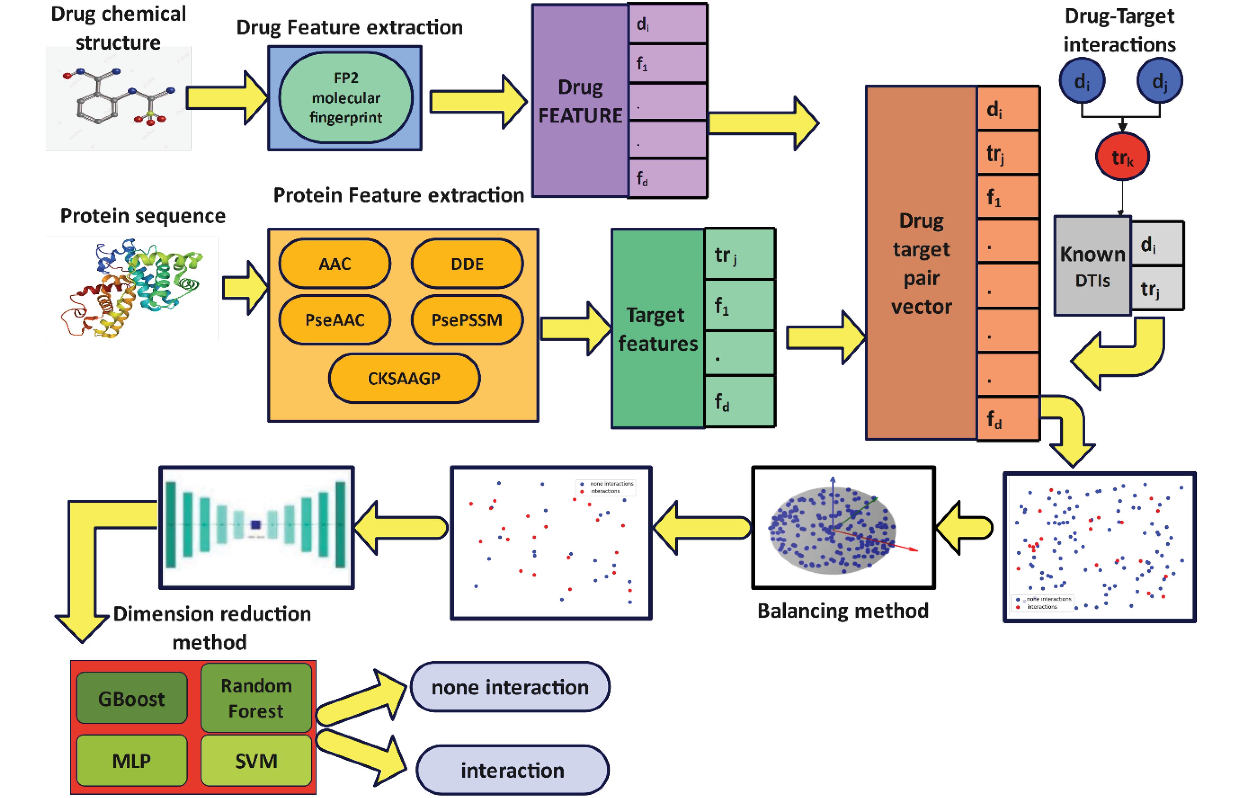
Fig. 1.
The workflow of the proposed model to predict drug-target interactions
.
The workflow of the proposed model to predict drug-target interactions
Feature extraction and composition
At this stage, due to the predication of drug-protein interactions, different features of drugs and proteins have been extracted. This feature extraction allows us to have a more detailed knowledge of interactions. In this section, we divide feature extraction into two categories:
Drug-related feature which includes fingerprints, and protein-related features that include AAC, DDE, PseAAC, PsePSSM, and CKSAAP features. In this paper, methods have been chosen to extract features from drugs and protein sequences, which show different aspects of the data. Then, the features extracted from drugs and proteins are combined with each other. If in the gold standard the pair of drug and protein interacts with each other, the label is assigned one; otherwise, zero is assigned. The study employed a comprehensive set of features categorized into drug and target groups. The drug feature group consisted of a molecular fingerprint with 256 features. For the target feature group, various types were utilized: Feature group A included 20 features based on amino acid composition (AAC); Feature group D comprised 400 features derived from dipeptide deviation from the expected mean (DDE); Feature group E contained 28 features related to pseudo amino acid composition (PseAAC); Feature group F included 220 features from the pseudo-position-specific scoring matrix (PsePSSM); and Feature group G encompassed 150 features based on the composition of k-spaced amino acid group pairs (CKSAAGP).
Data balancing
In this step, VASVDD_DTI method is used. This method is an unsupervised learning method to balance data in obstacles with unbalanced classes. In this method, a hypersphere is created, and this hypersphere should contain the most data with minimal comparison. Moreover, the points that are outside of this sphere are considered as noise or anomalies. Considering that the issue of predicting drug-protein interactions is an unbalanced data classification problem, that the data of one class (interaction between drug and protein) is less than the other class (non-interaction between drug and protein), In this paper, in the worst case, the ratio is one to one hundred. For this purpose, the paper aims to reduce the number of majority class data by using the improved VASVDD method.
In SVDD, all the features are used to build the supersphere because some features are extra, noisy, and unrelated. This makes the constructed supersphere not include the data that are representative of the majority class. Due to this, in the next phases, where the goal is to classify the data of two classes, machine learning models do not have an acceptable performance. However, to solve this problem, in this paper, a method is presented to create a supersphere by SVDD using encoder-decoder. Fig. 2 shows the general steps of the balancing method.
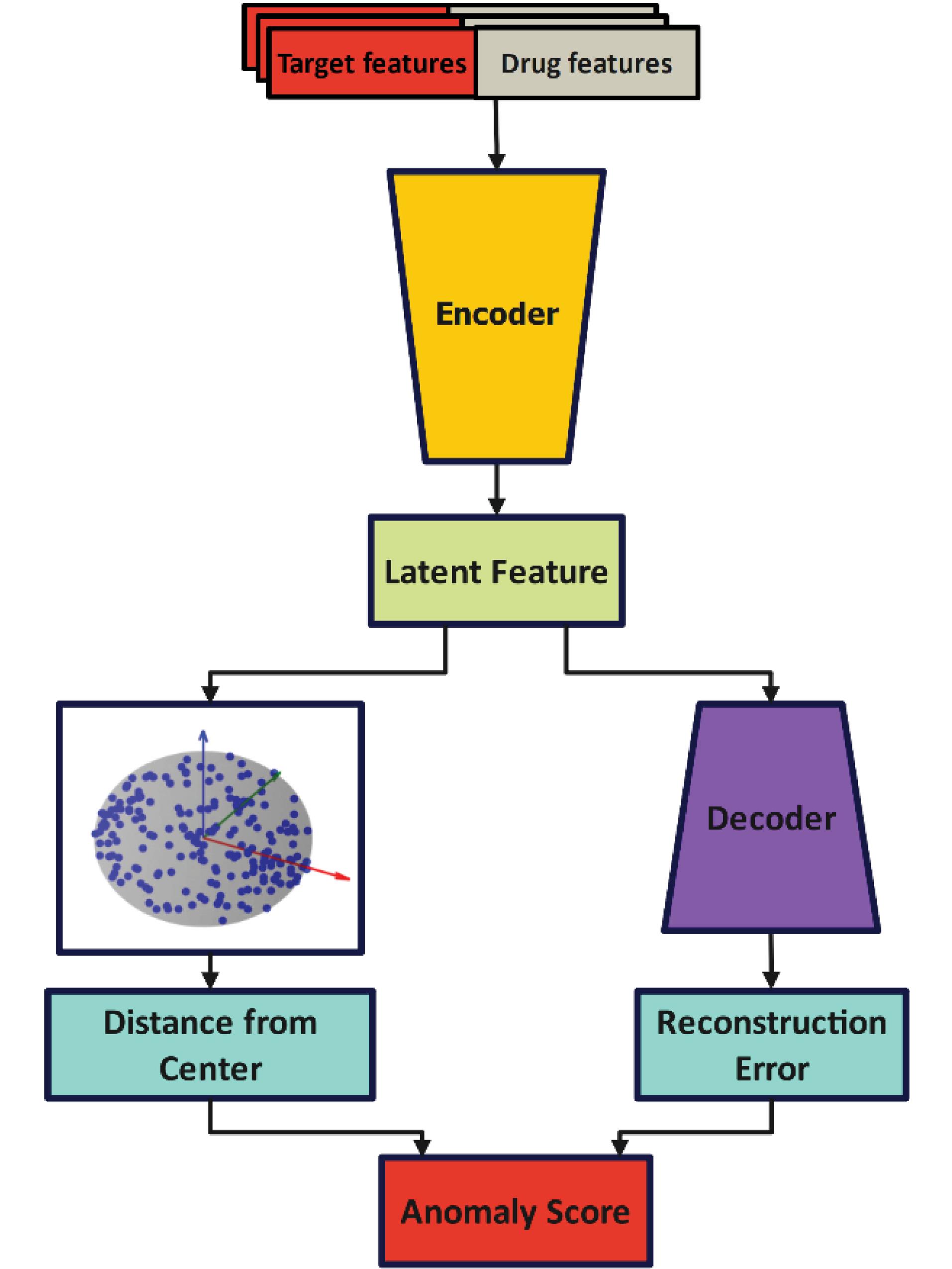
Fig. 2.
Proposed balancing model.
.
Proposed balancing model.
In this method, the characteristics of each data are considered as the input of the encoder. In the output layer of this encoder, the latent representation is specified for each data. This latent representation is a reduced dimensional version of the data that contains effective information from the data. In this step, this latent representation is used to construct the supersphere in SVDD. In this case, to demonstrate the appropriateness of this latent representation, a decoder has been used. At this stage, the encoder and decoder are in the form of h(.) and g(.) functions. The decoder takes the sample x and produces the latent representation z. z = h (x; θe) Therefore, this latent representation is used as input to the decoder to obtain the reconstructed output
. In these functions, θe and θd are the encoder and decoder parameters, respectively.
Subsequently, in order to build the supersphere with SVDD, the distance of the sample (latent representation) to the center of the supersphere is calculated. Therefore, by using the combination of the reconstruction error and the distance of the latent representation from the center of the hypersphere, the anomaly score of each sample x is calculated as equation (1).
(1)
In equation (1), c is the center of the supersphere, and γ is a superparameter that shows the balancing contribution of the two terms; hence, in order to find the appropriate data, we seek to minimize the following equation.
(2)
In equation (2), the first term is the reconstruction error, which specifies how our input data is made differently based on the encoder and decoder. The second term also shows the effect of latent representation in SVDD. Particularly, in the second term of the objective function, the goal is to build a hypersphere that includes only suitable data. Considering that the presented educational stage includes encoder and decoder training as well as building a supersphere, for this purpose in each stage, the data is divided into two parts. One part is used for training the center with the supersphere and one part is used for training θe and θd. The following equation is used to calculate the center. In this regard |B| is the size of the handle.
The latent representation of batch samples can be used to calculate the optimal center, which in equation (3), c is the center of the hypersphere and |B| is the size of the handle.
Reducing the dimensions of features
In general, after balancing the data of two classes, machine learning models are used to predict drug-protein interactions. However, due to the fact that the number of features of the data is large and it causes overfitting of machine learning models, it is necessary to identify the effective features.
At this stage, in order to prevent the increase of computing time, to increase the performance of classification models and to discover effective features, among all the features, dimensionality reduction based on VAE has been used.
The dimensional reduction model is based on VAE and is composed of two parts: encoder and decoder, which are also called transition functions and represented by f, g. Furthermore, x is considered as input data. By applying the transfer function f on the data, a latent representation z is constructed. In fact, this latent representation is a reduced version of the features. This representation is used as decoder input to reconstruct the data. Indeed, the more important the latent representation is, the more accurately the data is reconstructed. This latent representation, which is the output of the encoder, is used as dimensionality-reduced features.
Afterward, by applying the transfer function g, the data is reconstructed. equations (4), (5), and (6) clearly refer to it.
(6)
In the above equation, ψ and φ are encoder and decoder parameters,
is the reconstruction of the input vector
is the total error, which is calculated as the total reconstruction error of L in the dataset D.
Apart from this, VAE is used in this paper. VAE replaces deterministic functions in the encoder and decoder with stochastic mappings. Meanwhile, the objective function is calculated based on the density functions of random variables:
(7)
In equation (7), q is an approximating of the true latent distribution of z. φ, θ are considered as distribution parameters.
In the proposed method, there are 5 layers in the encoder phase. As previously mentioned, the first layer is the input. On the other hand, the reduction of these features in the next layer is clearly visible, so that the features are reduced from 1074 to 512. In the following, this process continues until it is reduced from 128 features to 64 in the last layer. As can be seen, the length of the obtained latent layer has 32 features and in the next phase, a decoder is used. This decoder, like the encoder, contains 5 layers, and its increasing trend is such that in the first layer, it has increased from 32 features to 64 features. this process will continue until it reconstructs the input by using the latent layer. As a result, in the last layer, the output has 1074 features. In the presented method, firstly, the model has been trained with epoch 20, then feature reduction has been done in the test phase. According to this paper, there are 1074 features of drugs and proteins, which were reduced to 32 by using dimension reduction methods. Fig. 3 shows the architecture of VAE.

Fig. 3.
The architecture of VAE.
.
The architecture of VAE.
Algorithm 1: Under Sampling by VASVDD
Input: X_train, c(0), θ0 =
, max_epochs, n, γ, κ
Output: c*, θ* =
1: Initialize Network Parameters θ = {θe, θd} and hyper-sphere center c
2: for each epoch in range(max_epochs) do
3: Select κ percent of the samples for the batch
4: Optimize θ for epoch (j + 1) to minimize the combined loss function:
5:
6: Select the remaining (1 - κ) percent of the samples
7: Optimize c for epoch (j + 1) to minimize the loss function:
8:
Predicting drug-protein interactions
After reducing the dimensions of the data, machine learning models are used to predict drug and protein interactions. For this purpose, first, the data is divided into two training and independent testing parts. In such a way that 20% of the total data is used as independent test and 80% as training and validation data. In order to better optimize parameters and calculate reliable results, the cross-validation method is used. It is noteworthy, in this essay, the value of K is equal to 5. Additionally, the classifier models include Gradient Boosting Classifier, Random Forest, SVM, and MPL.
Results
In this section, the proposed method is examined using various datasets and evaluated from multiple perspectives. The model is compared against existing models, focusing on two key aspects: balancing and dimensionality reduction. The results of this comparison demonstrate the superiority of the proposed model.
Data set
In this paper, four data related to enzymes (EN), Protein-coupled receptors (GPCR), ion channel (IC) and nuclear receptors (NR) published by Yamanishi et al9 have been used to predict drug-target interactions in the proposed model. This entire collection was retrieved from http://web.kuicr.kyoto-u.ac.jp/supp/yoshi/drugtarget/. Yamanishi et al9 have extracted information about drug-protein interactions from DrugBank,34 KEGG,32,33 BRENDA30 and Super Target.31 As a consequence, The study utilized several gold standard datasets, each with varying numbers of interactions, targets, and drugs. The EN dataset comprised 2,926 interactions involving 664 targets and 445 drugs. The GPCR dataset included 635 interactions with 95 targets and 223 drugs. The IC dataset consisted of 1476 interactions among 204 targets and 210 drugs. Lastly, the NR dataset contained 90 interactions with 26 targets and 54 drugs.
Evaluation criteria
In order to check the effectiveness of the proposed method, the criteria of accuracy, sensitivity, specificity and f1 score based on equations (8), (9), (10), (11) have been used.
In this paper, in discussing the composition of the extracted features, we utilized several feature extraction methods, including those mentioned in the article as well as additional methods like dipeptide composition and grouped amino acid composition. Through experiments conducted on the obtained data, we discovered that the combination of features from these six extraction methods yielded the best performance and achieved higher verified accuracy compared to other combinations. Additionally, our classifier demonstrated less bias towards the majority class. considering that the importance of the proposed work is balancing and reducing dimensions, the proposed method is examined from different aspects. In order to make the proposed method more effective, first, the extracted features are given to the Gradient Boosting Classifier (GBC) classification model without pre-processing and balancing. The results of this experiment are shown in Fig. 4.
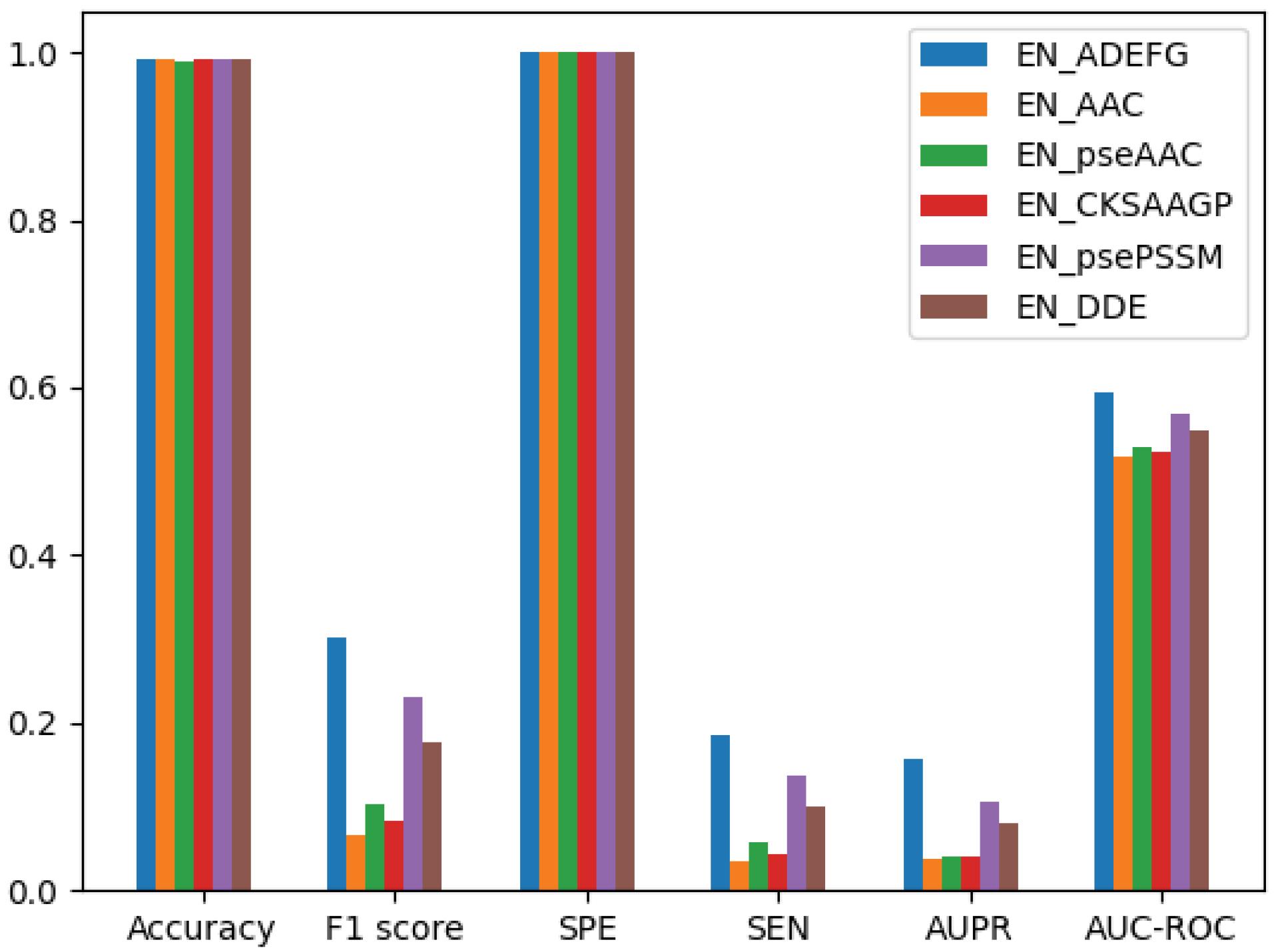
Fig. 4.
Bar chart of comparison between extracted and combined features.
.
Bar chart of comparison between extracted and combined features.
As it is clear from the results, the GBC model has an acceptable classification rate. Considering that the data of the two classes of the dataset used are clearly unbalanced, other criteria should be considered such as specificity and sensitivity. As it is obvious, the specificity has a good rate, but the sensitivity has a very low rate. This shows that the model has a low recognition rate in the classification of data with the minority class, but it predicts the majority class data well. This condition can be stated that the classification model is biased towards the majority of class. The combination of features can be used for causes a significant increase in sensitivity, f1 score, Area Under the Precision-Recall curve (AUPR) and Area Under the Receiver Operating Characteristic Curve (AUC-ROC), but it also shows the ability to use feature combination as a proposed method. consequently, Performance increases by using that.
In order to better analyze, Fig. 5 shows the confusion matrix of the GBC model for the EN dataset. As can be seen, the classifiers incorrectly predict the minority class (class 1) as the majority class (0). Fig. 5 shows the confusion matrix for the GBC bundle model based on the extracted features. Figure (a) is related to the combination of features, and (b) is related to the features extracted by the PseAAC method. As can be seen, machine learning models do not predict minority class samples well, in fact, the 463 data that should predict interaction are predicted. As can be seen, machine learning models do not predict minority class samples well, in fact, 463 of the data that should predict interaction predict as none interaction. Actually, the machine learning model is biased towards the majority class. The same problem exists in figure b, but the performance of the machine learning models is slightly improved when the feature combination is performed. Therefore, to increase the performance of machine learning methods, the data of two classes should be balanced.
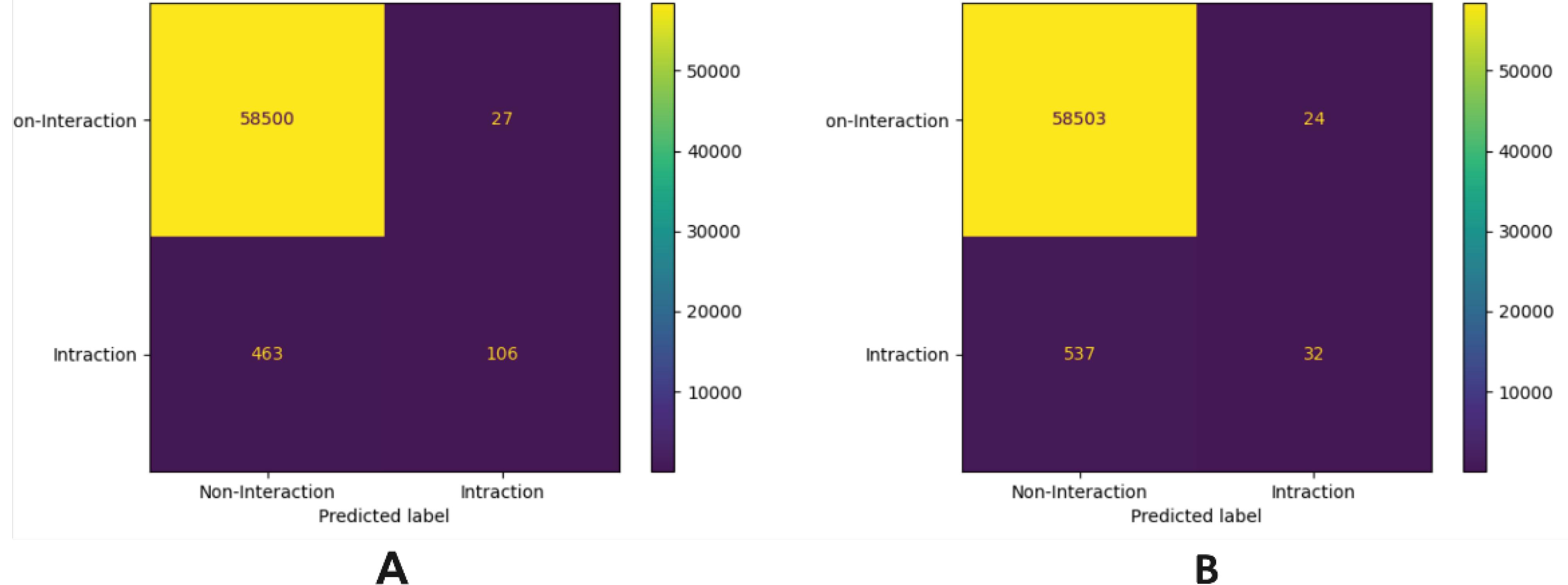
Fig. 5.
The confusion matrix of GBC A) training based on combined features, B) training based on PseAAC features.
.
The confusion matrix of GBC A) training based on combined features, B) training based on PseAAC features.
Analysis of data balancing methods
In order to investigate balance methods and their effect on the performance of classification methods, Table 1 shows the results of GBC on balanced data for different datasets. Undoubtedly, unlike when balancing is not done, in this case the classification model has an acceptable performance in all criteria such as accuracy, sensitivity, specificity and f1 score. It is clear that the model predicts the data of two classes significantly based on the criteria of specificity and sensitivity. Hence, it is not biased towards any class. The reason for increasing the efficiency of removing is outlier and noisy data from the majority class. In addition, the data which obtained in two classes have considerable distinctive features. Along with this, in order to evaluate the performance of the proposed method, it has been compared with other common balancing methods such as Synthetic Minority Oversampling Technique (SMOTE), Edited Nearest Neighbors (ENN), random under-sampling and random over-sampling. Although the proposed method performs more significant in comparison with other methods in all evaluation criteria, the only model that can compete with the proposed method is the ENN method.
Table 1.
Compare between the proposed balancing method with other methods
|
Dataset
|
Sampling method
|
ACC
|
F1
|
SPE
|
SEN
|
| EN |
RandomOverSampler |
0.8826 |
0.1245 |
0.8835 |
0.8016 |
| RandomUnderSampler |
0.8472 |
0.1032 |
0.8471 |
0.8538 |
| EditedNearestNeighbours |
0.9914 |
0.3389 |
0.9988 |
0.2288 |
| SMOTE |
0.9364 |
0.1704 |
0.9388 |
0.6819 |
| SVDD Deep |
0.9977
|
0.9929 |
1 |
0.9860 |
| GPCR |
RandomOverSampler |
0.8690 |
0.2127 |
0.8759 |
0.6302 |
| RandomUnderSampler |
0.7679 |
0.2040 |
0.7666 |
0.8025 |
| EditedNearestNeighbours |
0.9702 |
0.2921 |
0.9963 |
0.1897 |
| SMOTE |
0.9676 |
0.3800 |
0.9859 |
0.3471 |
| SVDD Deep |
0.9868
|
0.9650 |
0.9967 |
0.9452 |
| IC |
RandomOverSampler |
0.8574 |
0.2830 |
0.8580 |
0.8426 |
| RandomUnderSampler |
0.8036 |
0.2305 |
0.8021 |
0.8456 |
| EditedNearestNeighbours |
0.9687 |
0.3092 |
0.9957 |
0.2137 |
| SMOTE |
0.9363 |
0.3550 |
0.9498 |
0.5376 |
| SVDD Deep |
0.9905
|
0.9729 |
0.9959 |
0.9664 |
| NR |
RandomOverSampler |
0.9323 |
0.5581 |
0.9398 |
0.8 |
| RandomUnderSampler |
0.7259 |
0.3063 |
0.7276 |
0.7083 |
| EditedNearestNeighbours |
0.9252 |
0.4615 |
0.9436 |
0.6 |
| SMOTE |
0.9217 |
0.3125 |
0.9806 |
0.2272 |
| SVDD Deep |
0.9537
|
0.8484 |
0.9888 |
0.7777 |
Considering that a deep neural network is used in the proposed model, for this reason, the convergence process of the proposed method is shown in Fig. 6 of the loss diagram for different datasets. As it is known, the proposed method reduces the amount of loss decreases during the training process.
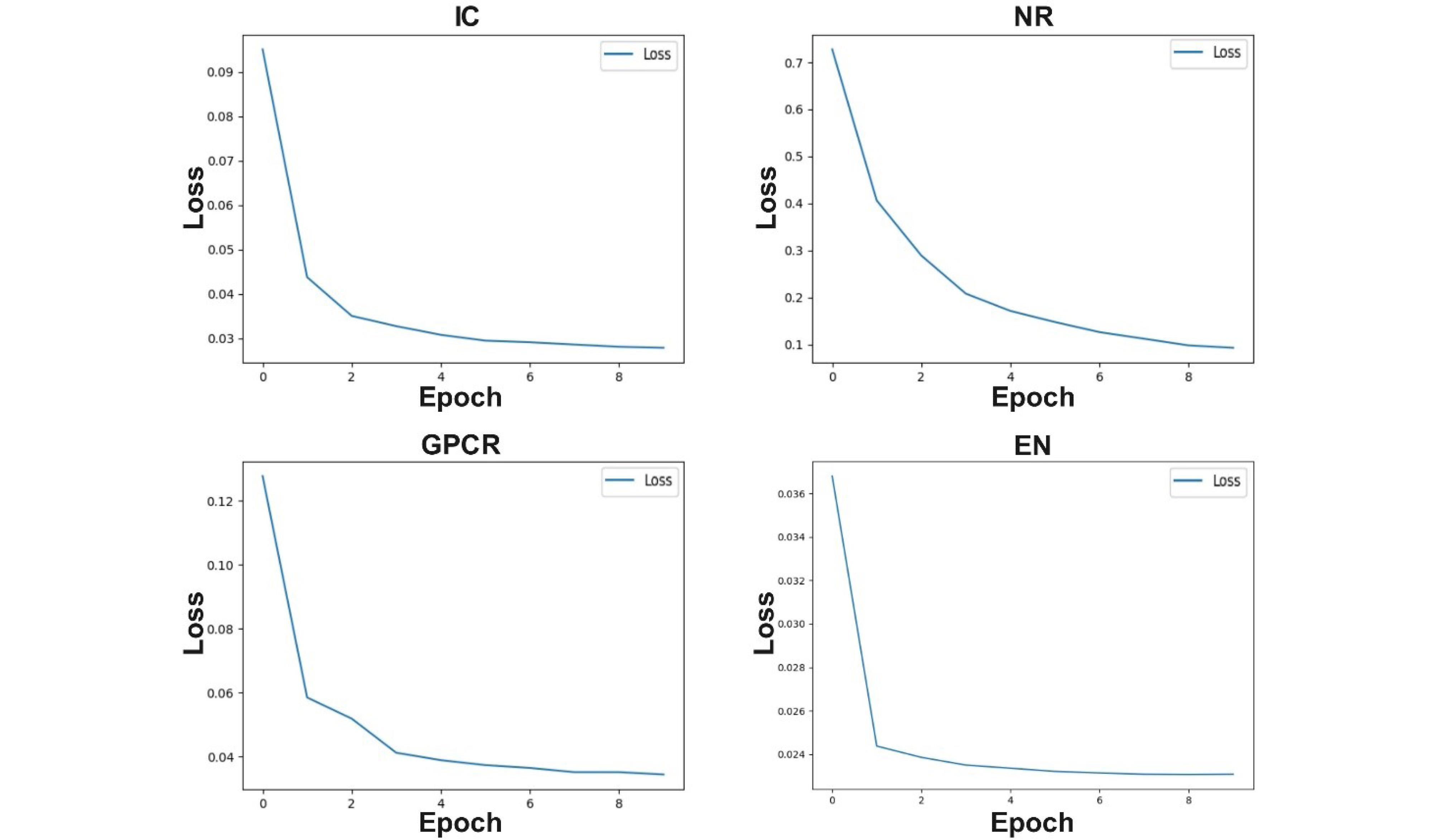
Fig. 6.
Loss value of the proposed balancing model on different datasets.
.
Loss value of the proposed balancing model on different datasets.
Analysis of the dimension reduction method
At this stage, after balancing the data to increase the efficiency of the classification models, according to the high number of features, the features are reduced using the Variational autoencoder method, then they are given to the classification models. The results are shown in Table 2. As is clear, the results are improved compared to the balancing mode. Dimensionality reduction has been done in EN, IC, GPCR and NR datasets using a variational autoencoder model subsequently so that the number of features has been reduced from 1074 to 32 features in each dataset. However, by using the GBC, the performance of the proposed model was evaluated in terms of accuracy, AUROC, AUPR and etc. Also, in order to ensure the efficiency of the proposed model, using the GBC, the obtained results, which are before and after dimension reduction in EN, IC, GPCR, and NR datasets, are compared using the accuracy measurement criteria.
Table 2.
Performance of the different classifiers without and with dimensionality reduction method
|
Dataset
|
Classifier
|
Dimension reduction
|
AUROC
|
AUPR
|
ACC
|
SEN
|
SPE
|
F1
|
| EN |
GBoost |
without |
0.9930 |
0.9882 |
0.9977 |
0.9860 |
1 |
0.9929 |
| with |
1 |
1 |
1 |
1 |
1 |
1 |
| MLP |
without |
0.9767 |
0.9496 |
0.9906 |
0.9562 |
0.9972 |
0.9707 |
| with |
0.9981 |
0.9881 |
0.9980 |
0.9982 |
0.9979 |
0.9939 |
| RF |
without |
0.9903 |
0.9839 |
0.9968 |
0.9807 |
1 |
0.9902 |
| with |
1 |
1 |
1 |
1 |
1 |
1 |
| SVM |
without |
0.9152 |
0.8508 |
0.9712 |
0.8321 |
0.9982 |
0.9040 |
| with |
0.9851 |
0.9515 |
0.9911 |
0.9761 |
0.9941 |
0.9736 |
| GPCR |
GBoost |
without |
0.9709 |
0.9422 |
0.9868 |
0.9452 |
0.9967 |
0.9650 |
| with |
1 |
1 |
1 |
1 |
1 |
1 |
| MLP |
without |
0.8463 |
0.6330 |
0.9120 |
0.7397 |
0.9529 |
0.7632 |
| with |
0.9856 |
0.9502 |
0.9895 |
0.9794 |
0.9918 |
0.9727 |
| RF |
without |
0.9520 |
0.9224 |
0.9816 |
0.9041 |
1 |
0.9496 |
| with |
1 |
1 |
1 |
1 |
1 |
1 |
| SVM |
without |
0.6564 |
0.3883 |
0.8543 |
0.3356 |
0.9772 |
0.4688 |
| with |
0.9183 |
0.8087 |
0.9566 |
0.8561 |
0.9805 |
0.8833 |
| NR |
GBoost |
without |
0.8833 |
0.7629 |
0.9537 |
0.7777 |
0.9888 |
0.8484 |
| with |
1 |
1 |
1 |
1 |
1 |
1 |
| MLP |
without |
0.7234 |
0.3564 |
0.8888 |
0.5 |
0.9468 |
0.5384 |
| with |
0.9483 |
0.7637 |
0.9629 |
0.9285 |
0.9680 |
0.8666 |
| RF |
without |
0.8571 |
0.7513 |
0.9629 |
0.7142 |
1 |
0.8333 |
| with |
1 |
1 |
1 |
1 |
1 |
1 |
| SVM |
without |
0.6572 |
0.2817 |
0.8796 |
0.3571 |
0.9574 |
0.4347 |
| with |
0.8465 |
0.6322 |
0.9444 |
0.7142 |
0.9787 |
0.7692 |
| IC |
GBoost |
without |
0.9811 |
0.9523 |
0.9905 |
0.9664 |
0.9959 |
0.9729 |
| with |
1 |
1 |
1 |
1 |
1 |
1 |
| MLP |
without |
0.9102 |
0.7535 |
0.9505 |
0.8489 |
0.9715 |
0.8532 |
| with |
0.9888 |
0.9599 |
0.9926 |
0.9832 |
0.9945 |
0.9782 |
| RF |
without |
0.9661 |
0.9408 |
0.9881 |
0.9328 |
0.9993 |
0.9636 |
| with |
1 |
1 |
1 |
1 |
1 |
1 |
| SVM |
without |
0.7687 |
0.5799 |
0.9159 |
0.5469 |
0.9905 |
0.6863 |
| with |
0.9378 |
0.8454 |
0.9700 |
0.8892 |
0.9864 |
0.9090 |
The results show that, in the EN dataset, accuracy increased from 0.9977 to 1, in the GPCR dataset from 0.9868 to 1, in the NR dataset from 0.9537 to 1, and in the IC dataset from 0.9905 to 1. Admittedly, the results did not increase incrementally. With this in mind, in the previous stage, in the VASVDD model, the features have been selected and the proposed model in that has balanced the data based on the selected features.
In order to investigate dimension reduction methods and its impact on the performance of classification methods, the results of GBC classification on dimensionality reduction data are shown in Fig. 7 for different datasets. Obviously, when the dimensions are reduced, in this case, the classification model has an acceptable performance in all criteria such as Accuracy (ACC), Sensitivity (SEN), Specificity (SPE), and F1 score (F1). The results show that the performance of the model has improved compared to before the implementation of dimension reduction. In order to evaluate the performance of the dimension reduction method in the proposed method, this method has been compared with other common dimension reduction methods such as Kernel PCA, Non-Negative Matrix Factorization (NMF), Principal component analysis (PCA), truncated singular value decomposition (Truncated SVD) and FastUS.37 As is clear, the proposed method has better performance rather than other methods in all evaluation criteria The important point in this comparison is to pay attention to the values of specificity and sensitivity criteria in some methods. Some methods perform dimensionality reduction in such a way that the dimensionality-reduced data or data with new dimensions do not increase but decrease the performance of classification models, and the model will be biased towards the majority class. This means that in some methods, the obtained features do not have good distinguishing features in two classes.
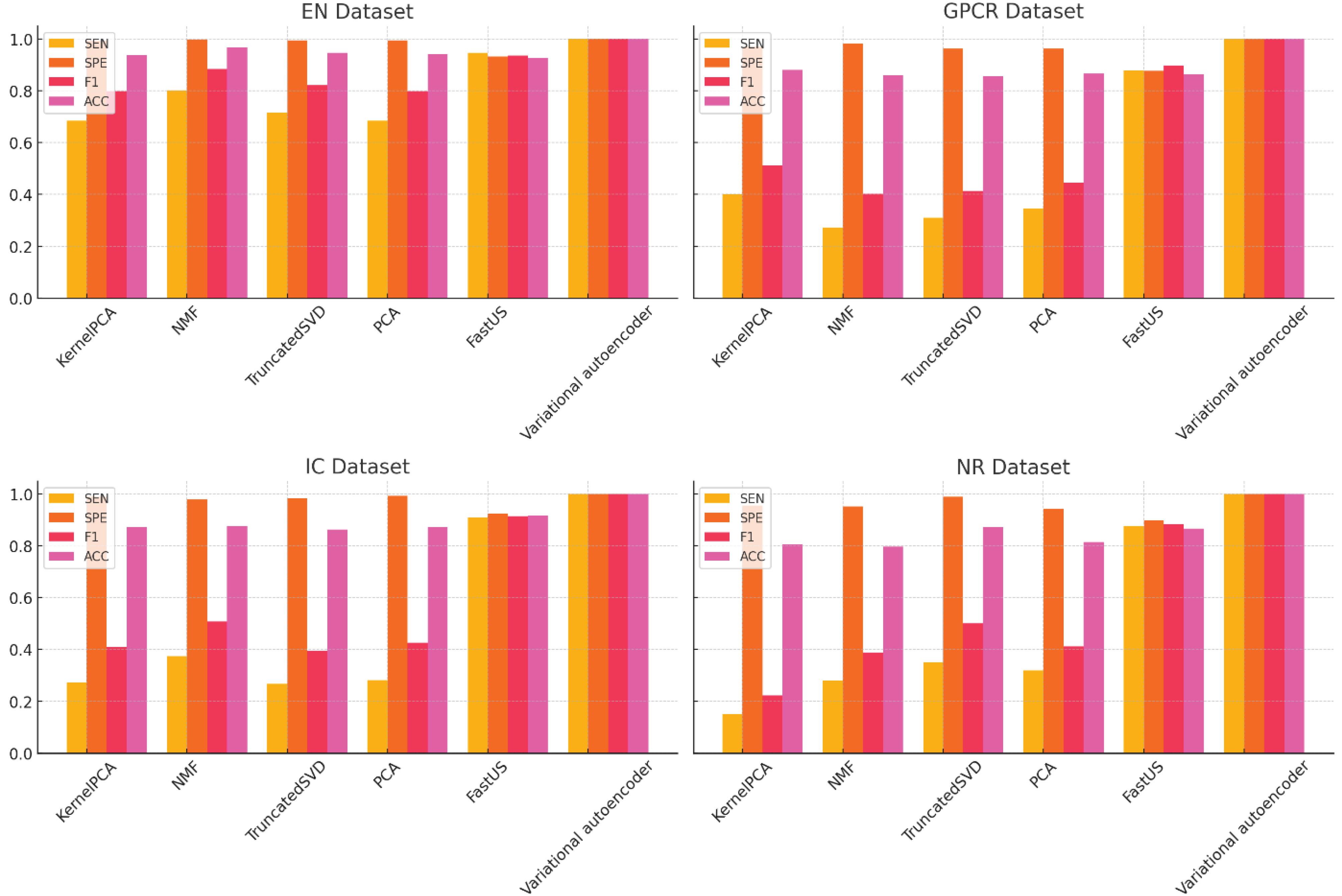
Fig. 7.
Compare the prediction results on balanced data using Variational autoencoder against other dimension reduction methods.
.
Compare the prediction results on balanced data using Variational autoencoder against other dimension reduction methods.
One of the important criteria in evaluating classification models is the use of the Receiver operating characteristic (ROC), which is performed on dimensionally reduced data. This curve shows the efficiency of the proposed method, and in other words, it determines the false positive value of the classification model. In this case, the greater the area under the curve, show the more effective the proposed method. Fig. 8, show the ROC of the proposed method based on different classifiers. As it is known, the area under the ROC of the proposed model is high in all datasets for different classifiers. This shows that the proposed model is not dependent on the classifier, and its performance is acceptable in all various classifiers.
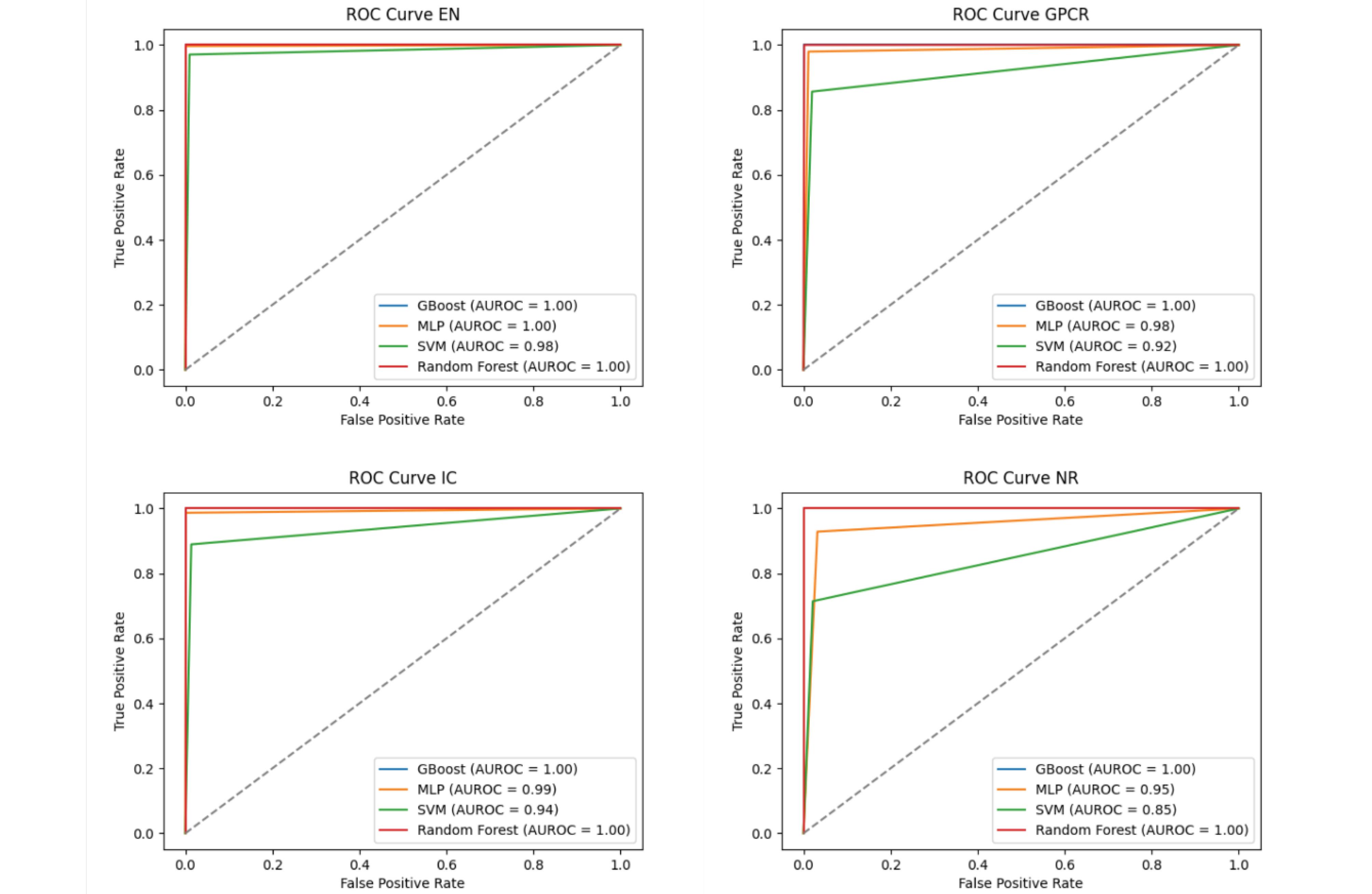
Fig. 8.
ROC curves of the proposed method with different machine learning models on different datasets.
.
ROC curves of the proposed method with different machine learning models on different datasets.
The variance of the proposed method in Accuracy values is shown in Table 3. As can be seen, EN, IC, GPCR, and NR datasets have been checked using Random Forest, support vector machines (SVM), multilayer perceptron (MLP), and GBC classification methods in k-fold cross-validation with k = 5. Particularly, by using the mentioned classifiers, their average and variance have also been obtained. In addition to this, the average is close to the Accuracy, and the variance of the proposed method is low. This shows the optimal performance of the proposed method.
Table 3.
Comparison of Accuracy values under the 5-Fold cross-validation on datasets
|
|
Datasets
|
|
|
EN
|
GPCR
|
|
Fold
|
GBOOST
|
MLP
|
RF
|
SVM
|
GBOOST
|
MLP
|
RF
|
SVM
|
| 1 |
1 |
0.9978 |
1 |
0.9882 |
1 |
0.9950 |
0.9983 |
0.9639 |
| 2 |
1 |
0.9953 |
1 |
0.9868 |
1 |
0.9885 |
0.9967 |
0.9655 |
| 3 |
1 |
0.9985 |
1 |
0.9886 |
1 |
0.9967 |
1 |
0.9688 |
| 4 |
0.9992 |
0.9967 |
1 |
0.9882 |
1 |
0.9950 |
1 |
0.9786 |
| 5 |
0.9996 |
0.9975 |
1 |
0.9857 |
0.9983 |
0.9901 |
1 |
0.9720 |
| Mean |
0.9997 |
0.9972 |
1 |
0.9875 |
0.9996 |
0.9931 |
0.9990 |
0.9698 |
| Std |
0.0002 |
0.001 |
0.0 |
0.0010 |
0.0006 |
0.0031 |
0.0013 |
0.0052 |
|
|
IC
|
NR
|
|
Fold
|
GBOOST
|
MLP
|
RF
|
SVM
|
GBOOST
|
MLP
|
RF
|
SVM
|
| 1 |
1 |
0.9936 |
1 |
0.9781 |
1 |
0.9885 |
0.9885 |
0.8735 |
| 2 |
1 |
0.9964 |
1 |
0.9738 |
1 |
0.9540 |
1 |
0.8965 |
| 3 |
1 |
0.9943 |
1 |
0.9788 |
1 |
1 |
0.9767 |
0.8837 |
| 4 |
1 |
0.9957 |
1 |
0.9604 |
1 |
0.9767 |
0.9883 |
0.9186 |
| 5 |
1 |
0.9950 |
1 |
0.9618 |
1 |
0.9883 |
1 |
0.8720 |
| Mean |
1 |
0.9950 |
1 |
0.9706 |
1 |
0.9815 |
0.9907 |
0.8889 |
| Std |
0.0 |
0.0009 |
0.0 |
0.0079 |
0.0 |
0.0155 |
0.0086 |
0.0172 |
Comparison of the proposed method with other methods
In recent years, various methods have been proposed to predict DTIs in the form of machine learning. Most of the methods are used from the dataset proposed by Yamanishi et al.9 In order to show the effectiveness of the proposed method, it is compared with other methods using the AUROC evaluation criterion. The results of this comparison are given in Table 4. As can be seen, the AUROC of the proposed model is superior to other methods.
Table 4.
Comparison of proposed model with existing methods on four datasets
|
Dataset
|
Mousavian et al
21
|
Li Z et al
23
|
Meng et al
35
|
Wang et al
29
|
Mahmud et al
4
|
Wang et al
36
|
Mahmud et al
37
|
Khojasteh et al
13
|
Proposed method
|
| EN |
0.9480 |
0.9288 |
0.9773 |
0.9150 |
0.9808 |
0.9172 |
0.9656 |
0.9920 |
1 |
| IC |
0.8890 |
0.9171 |
0.9312 |
0.8900 |
0.9727 |
0.8827 |
0.9612 |
0.9880 |
1 |
| GPCR |
0.8720 |
0.8856 |
0.8677 |
0.8450 |
0.9390 |
0.8557 |
0.9249 |
0.9788 |
1 |
| NR |
0.8690 |
0.9300 |
0.8778 |
0.7230 |
0.9198 |
0.7531 |
0.8652 |
0.9329 |
0.968 |
The AUROC values in the proposed model were obtained in all datasets using the GBC model. The proposed model demonstrates high generalizability, as it achieves superior performance with only 32 features compared to using all 1074 features. This not only improves the computational efficiency but also makes the model compatible with various classification methods, including XGBoost, GBC, and random forest, allowing these classifiers to perform effectively in predicting DTIs.
The model was evaluated using a subset of data from four different datasets designated as independent test sets to ensure unbiased performance assessment. The results demonstrated high accuracy, especially in scenarios involving new drugs and new targets, proving the model's robustness and effectiveness in drug discovery and development. The performance of different datasets evaluated using accuracy (ACC) is as follows. The EN_ADEFG dataset achieved an accuracy of 0.9943. The IC_ADEFG dataset performed slightly better with an accuracy of 0.9962. The GPCR_ADEFG dataset showed the highest accuracy at 0.9986. Finally, the NR_ADEFG dataset had an accuracy of 0.9649.
Conclusion
In this paper, a four-step method for Predicting drug-protein interactions is presented. These steps include feature extraction, data balancing, data dimensionality reduction and classification. For this purpose, Respectively, SVDD deep and VAE have been used to balance and reduce the dimensions of the data. The performance of the offending classifiers has been evaluated on different datasets and the results indicate that the proposed model is not dependent on the classification methods and the balancing has been executed effectively.
In addition, the results demonstrate that the proposed method outperforms other balancing methods. Furthermore, this method proves to be more effective than other methods in the field of drug-protein interaction prediction.
Research Highlights
What is the current knowledge?
-
Machine learning methods predict drug-target interactions with varying success.
-
Class imbalance and high-dimensional data pose significant challenges.
-
Techniques like SMOTE and ENN address class imbalance issues.
-
Dimensionality reduction methods like PCA and Kernel PCA manage high-dimensional data.
-
Traditional methods often struggle with accuracy and generalizability.
What is new here?
-
Introduced VASVDD for drug-target interaction prediction.
-
Evaluated VASVDD on multiple standard databases.
-
Demonstrated superior performance over state-of-the-art methods.
-
Improved prediction accuracy and robustness in drug-protein interactions.
-
Achieved better generalizability and computational efficiency across datasets.
Competing Interests
The authors declare no competing interests.
Ethical Statement
Not applicable.
References
- Cao DS, Liu S, Xu QS, Lu HM, Huang JH, Hu QN. Large-scale prediction of drug-target interactions using protein sequences and drug topological structures. Anal Chim Acta 2012; 752:1-10. doi: 10.1016/j.aca.2012.09.021 [Crossref] [ Google Scholar]
- Zhao ZY, Huang WZ, Zhan XK, Huang YA, Zhang SW, Yu CQ. Improved prediction of drug-target interactions based on ensemble learning with fuzzy local ternary pattern. Front Biosci (Landmark Ed) 2021; 26:222-34. doi: 10.52586/4936 [Crossref] [ Google Scholar]
- Redkar S, Mondal S, Joseph A, Hareesha KS. A machine learning approach for drug-target interaction prediction using wrapper feature selection and class balancing. Mol Inform 2020; 39:e1900062. doi: 10.1002/minf.201900062 [Crossref] [ Google Scholar]
- Mahmud SM, Chen W, Meng H, Jahan H, Liu Y, Hasan SM. Prediction of drug-target interaction based on protein features using undersampling and feature selection techniques with boosting. Anal Biochem 2020; 589:113507. doi: 10.1016/j.ab.2019.113507 [Crossref] [ Google Scholar]
- Keiser MJ, Roth BL, Armbruster BN, Ernsberger P, Irwin JJ, Shoichet BK. Relating protein pharmacology by ligand chemistry. Nat Biotechnol 2007; 25:197-206. doi: 10.1038/nbt1284 [Crossref] [ Google Scholar]
- Alsenan SA, Al-Turaiki IM, Hafez AM. Feature extraction methods in quantitative structure–activity relationship modeling: a comparative study. IEEE Access 2020; 8:78737-52. doi: 10.1109/access.2020.2990375 [Crossref] [ Google Scholar]
- Yu L, Qiu W, Lin W, Cheng X, Xiao X, Dai J. HGDTI: predicting drug-target interaction by using information aggregation based on heterogeneous graph neural network. BMC Bioinformatics 2022; 23:126. doi: 10.1186/s12859-022-04655-5 [Crossref] [ Google Scholar]
- Peska L, Buza K, Koller J. Drug-target interaction prediction: a Bayesian ranking approach. Comput Methods Programs Biomed 2017; 152:15-21. doi: 10.1016/j.cmpb.2017.09.003 [Crossref] [ Google Scholar]
- Yamanishi Y, Araki M, Gutteridge A, Honda W, Kanehisa M. Prediction of drug-target interaction networks from the integration of chemical and genomic spaces. Bioinformatics 2008; 24:i232-40. doi: 10.1093/bioinformatics/btn162 [Crossref] [ Google Scholar]
- Ballesteros J, Palczewski K. G protein-coupled receptor drug discovery: implications from the crystal structure of rhodopsin. Curr Opin Drug Discov Devel 2001; 4:561-74. [ Google Scholar]
- D'Souza S, Prema KV, Balaji S, Shah R. Deep learning-based modeling of drug-target interaction prediction incorporating binding site information of proteins. Interdiscip Sci 2023; 15:306-15. doi: 10.1007/s12539-023-00557-z [Crossref] [ Google Scholar]
- van Westen GJ, Wegner JK, Ijzerman AP, van Vlijmen HW, Bender A. Proteochemometric modeling as a tool to design selective compounds and for extrapolating to novel targets. Med Chem Commun 2011; 2:16-30. doi: 10.1039/c0md00165a [Crossref] [ Google Scholar]
- Khojasteh H, Pirgazi J, Ghanbari Sorkhi A. Improving prediction of drug-target interactions based on fusing multiple features with data balancing and feature selection techniques. PLoS One 2023; 18:e0288173. doi: 10.1371/journal.pone.0288173 [Crossref] [ Google Scholar]
- Gfeller D, Grosdidier A, Wirth M, Daina A, Michielin O, Zoete V. SwissTargetPrediction: a web server for target prediction of bioactive small molecules. Nucleic Acids Res 2014; 42:W32-8. doi: 10.1093/nar/gku293 [Crossref] [ Google Scholar]
- Shi JY, Yiu SM, Li Y, Leung HC, Chin FY. Predicting drug-target interaction for new drugs using enhanced similarity measures and super-target clustering. Methods 2015; 83:98-104. doi: 10.1016/j.ymeth.2015.04.036 [Crossref] [ Google Scholar]
- Lim H, Gray P, Xie L, Poleksic A. Improved genome-scale multi-target virtual screening via a novel collaborative filtering approach to cold-start problem. Sci Rep 2016; 6:38860. doi: 10.1038/srep38860 [Crossref] [ Google Scholar]
- Rifaioglu AS, Atas H, Martin MJ, Cetin-Atalay R, Atalay V, Doğan T. Recent applications of deep learning and machine intelligence on in silico drug discovery: methods, tools and databases. Brief Bioinform 2019; 20:1878-912. doi: 10.1093/bib/bby061 [Crossref] [ Google Scholar]
- Ding H, Takigawa I, Mamitsuka H, Zhu S. Similarity-based machine learning methods for predicting drug-target interactions: a brief review. Brief Bioinform 2014; 15:734-47. doi: 10.1093/bib/bbt056 [Crossref] [ Google Scholar]
- Pahikkala T, Airola A, Pietilä S, Shakyawar S, Szwajda A, Tang J. Toward more realistic drug-target interaction predictions. Brief Bioinform 2015; 16:325-37. doi: 10.1093/bib/bbu010 [Crossref] [ Google Scholar]
- Nascimento AC, Prudêncio RB, Costa IG. A multiple kernel learning algorithm for drug-target interaction prediction. BMC Bioinformatics 2016; 17:46. doi: 10.1186/s12859-016-0890-3 [Crossref] [ Google Scholar]
- Mousavian Z, Khakabimamaghani S, Kavousi K, Masoudi-Nejad A. Drug-target interaction prediction from PSSM based evolutionary information. J Pharmacol Toxicol Methods 2016; 78:42-51. doi: 10.1016/j.vascn.2015.11.002 [Crossref] [ Google Scholar]
- LeCun Y, Bengio Y, Hinton G. Deep learning. Nature 2015; 521:436-44. doi: 10.1038/nature14539 [Crossref] [ Google Scholar]
- Li Z, Han P, You ZH, Li X, Zhang Y, Yu H. In silico prediction of drug-target interaction networks based on drug chemical structure and protein sequences. Sci Rep 2017; 7:11174. doi: 10.1038/s41598-017-10724-0 [Crossref] [ Google Scholar]
- Rayhan F, Ahmed S, Shatabda S, Farid DM, Mousavian Z, Dehzangi A. iDTI-ESBoost: identification of drug target interaction using evolutionary and structural features with boosting. Sci Rep 2017; 7:17731. doi: 10.1038/s41598-017-18025-2 [Crossref] [ Google Scholar]
- Jiang J, Wang N, Chen P, Zhang J, Wang B. DrugECs: an ensemble system with feature subspaces for accurate drug-target interaction prediction. Biomed Res Int 2017; 2017:6340316. doi: 10.1155/2017/6340316 [Crossref] [ Google Scholar]
- Mahmud SM, Chen W, Jahan H, Liu Y, Sujan NI, Ahmed S. iDTi-CSsmoteB: identification of drug–target interaction based on drug chemical structure and protein sequence using XGBoost with over-sampling technique SMOTE. IEEE Access 2019; 7:48699-714. doi: 10.1109/access.2019.2910277 [Crossref] [ Google Scholar]
- Shi H, Liu S, Chen J, Li X, Ma Q, Yu B. Predicting drug-target interactions using Lasso with random forest based on evolutionary information and chemical structure. Genomics 2019; 111:1839-52. doi: 10.1016/j.ygeno.2018.12.007 [Crossref] [ Google Scholar]
- Rayhan F, Ahmed S, Mousavian Z, Farid DM, Shatabda S. FRnet-DTI: deep convolutional neural network for drug-target interaction prediction. Heliyon 2020; 6:e03444. doi: 10.1016/j.heliyon.2020.e03444 [Crossref] [ Google Scholar]
- Wang L, You ZH, Chen X, Yan X, Liu G, Zhang W. RFDT: a rotation forest-based predictor for predicting drug-target interactions using drug structure and protein sequence information. Curr Protein Pept Sci 2018; 19:445-54. doi: 10.2174/1389203718666161114111656 [Crossref] [ Google Scholar]
- Schomburg I, Chang A, Ebeling C, Gremse M, Heldt C, Huhn G. BRENDA, the enzyme database: updates and major new developments. Nucleic Acids Res 2004; 32:D431-3. doi: 10.1093/nar/gkh081 [Crossref] [ Google Scholar]
- Günther S, Kuhn M, Dunkel M, Campillos M, Senger C, Petsalaki E. SuperTarget and Matador: resources for exploring drug-target relationships. Nucleic Acids Res 2008; 36:D919-22. doi: 10.1093/nar/gkm862 [Crossref] [ Google Scholar]
- Kanehisa M, Goto S, Hattori M, Aoki-Kinoshita KF, Itoh M, Kawashima S. From genomics to chemical genomics: new developments in KEGG. Nucleic Acids Res 2006; 34:D354-7. doi: 10.1093/nar/gkj102 [Crossref] [ Google Scholar]
- Kanehisa M, Goto S, Sato Y, Furumichi M, Tanabe M. KEGG for integration and interpretation of large-scale molecular data sets. Nucleic Acids Res 2012; 40:D109-14. doi: 10.1093/nar/gkr988 [Crossref] [ Google Scholar]
- Wishart DS, Knox C, Guo AC, Shrivastava S, Hassanali M, Stothard P. DrugBank: a comprehensive resource for in silico drug discovery and exploration. Nucleic Acids Res 2006; 34:D668-72. doi: 10.1093/nar/gkj067 [Crossref] [ Google Scholar]
- Meng FR, You ZH, Chen X, Zhou Y, An JY. Prediction of drug-target interaction networks from the integration of protein sequences and drug chemical structures. Molecules 2017; 22:1119. doi: 10.3390/molecules22071119 [Crossref] [ Google Scholar]
- Wang Y, Wang L, Wong L, Zhao B, Su X, Li Y. RoFDT: identification of drug-target interactions from protein sequence and drug molecular structure using rotation forest. Biology (Basel) 2022; 11:741. doi: 10.3390/biology11050741 [Crossref] [ Google Scholar]
- Mahmud SM, Chen W, Liu Y, Awal MA, Ahmed K, Rahman MH. PreDTIs: prediction of drug-target interactions based on multiple feature information using gradient boosting framework with data balancing and feature selection techniques. Brief Bioinform 2021; 22:bbab046. doi: 10.1093/bib/bbab046 [Crossref] [ Google Scholar]